Optimzing our LLM RL Pipeline

Optimzing our LLM RL Pipeline#

For part of our work on applying reinforcmenent learning to LLMs at Berkeley, I wanted to write a minimal version of an RL loop that prioritizes ease-of-research. But we need to make sure that experiments still run fast! In this post, I’ll focus specifically on the performance optimizations that underline the efficiency of our library, Language Model Policy Optimization.

As LMPO is a JAX codebase, the specific tools we’ll be using will be native to JAX and the TPU ecosystem. We conducted these experiments on a v4-32 TPU pod, courtesy of the TPU Research Cloud.

Baseline: Qwen3-1.7B with unified inference/training graph#

As a base model, we will keep things simple and use an off-the-shelf Qwen3 model. To load the Qwen model into Jax, we will need to re-define the network graph in terms of Flax modules. We’ll also want to include support for a KV (key-value) cache, since we will be using this model for both sampling and training.

In a lot of RL systems, the frameworks used for training and sampling are completely different. For example, a common setup is to use vLLM or SGLang for sampling, and then train the model with a separate set of code. This means defining the network pass twice, which can possibly lead to mismatches in inference and train-time (). For our minimal library, I wanted to use the same graph for both inference and training. This makes it easy to launch end-to-end experiments on any set of TPUs, without needing to split them into specialized sampling or training workers.

It is not complicated to re-implement transformer models. Click into the dropdown below to read the model code for a single layer:

Show code cell content Hide code cell content

class Block(nn.Module):
    """ A standard transformer block. Has residual connection, self-attention, and a two-layer MLP. """
    hidden_size: int
    q_heads: int
    kv_heads: int
    head_dim: int
    mlp_ffw_size: int
    eps: float = 1e-6

    @nn.compact
    def __call__(self, x, sin, cos, token_mask, layer_id, cache=None):

        # =========================
        # === Self-Attention Block. 
        # =========================

        pre_gamma = self.param('pre_gamma', nn.initializers.constant(1.0), (self.hidden_size,))
        x_norm = rms_norm(x, pre_gamma, self.eps)
        
        # Calculate Q,K,V.
        q = nn.Dense(self.q_heads * self.head_dim, use_bias=False, dtype=jnp.bfloat16)(x_norm)
        q = jnp.reshape(q, (q.shape[0], q.shape[1], self.q_heads, self.head_dim))
        k = nn.Dense(self.kv_heads * self.head_dim, use_bias=False, dtype=jnp.bfloat16)(x_norm)
        k = jnp.reshape(k, (k.shape[0], k.shape[1], self.kv_heads, self.head_dim))
        v = nn.Dense(self.kv_heads * self.head_dim, use_bias=False, dtype=jnp.bfloat16)(x_norm)
        v = jnp.reshape(v, (v.shape[0], v.shape[1], self.kv_heads, self.head_dim))

        q_gamma = self.param('q_gamma', nn.initializers.constant(1.0), (self.head_dim,))
        q = rms_norm(q, q_gamma, self.eps)
        q = apply_rotary_embedding(q, sin, cos)
        k_gamma = self.param('k_gamma', nn.initializers.constant(1.0), (self.head_dim,))
        k = rms_norm(k, k_gamma, self.eps)
        k = apply_rotary_embedding(k, sin, cos)
        q_idx, k_idx = token_mask, token_mask

        # Causal Attention Mask.
        b, t, qh, d = q.shape # qh = 16
        _, T, kh, _ = k.shape # kh = 8
        mask = q_idx[:, :, None] & k_idx[:, None, :]
        mask = mask[:, None, :, :] # [B, 1, t, T]
        qk_size = (1, 1, t, T)
        q_iota = jax.lax.broadcasted_iota(jnp.int32, qk_size, 2)
        k_iota = jax.lax.broadcasted_iota(jnp.int32, qk_size, 3)
        q_positions = q_iota
        causal_mask = q_positions >= k_iota
        mask = jnp.logical_and(mask, causal_mask)
        mask = jnp.transpose(mask, (0, 2, 3, 1)) # [B, t, T, 1]

        if cache is not None:
            k = jax.lax.dynamic_update_slice_in_dim(cache.k[layer_id], k, cache.length, axis=1)
            v = jax.lax.dynamic_update_slice_in_dim(cache.v[layer_id], v, cache.length, axis=1)
            cache.k[layer_id] = k
            cache.v[layer_id] = v

        # Attention.
        q = jnp.reshape(q, (b, t, kh, qh // kh, d))
        qk = jnp.einsum("bthgd,bThd->btThg", q, k) * (d ** -0.5)
        qk = jnp.reshape(qk, (b, t, T, qh)) 
        qk = jnp.where(mask, qk, -1e30) # good
        attn = jax.nn.softmax(qk.astype(jnp.float32), axis=2) # on T dimension.
        attn = jnp.reshape(attn, (b, t, T, kh, qh // kh))
        qkv = jnp.einsum("btThg,bThd->bthgd", attn, v).astype(x.dtype)
        qkv = jnp.reshape(qkv, (b, t, qh*d))
        attn_x = nn.Dense(self.hidden_size, use_bias=False, dtype=jnp.bfloat16)(qkv)
        x = x + attn_x
        
        # =========================
        # === MLP Block. 
        # =========================
        post_gamma = self.param('post_gamma', nn.initializers.constant(1.0), (self.hidden_size,))
        x_norm = rms_norm(x, post_gamma, self.eps)
        g = nn.Dense(features=self.mlp_ffw_size, use_bias=False, dtype=jnp.bfloat16)(x_norm)
        g = nn.silu(g)
        y = nn.Dense(features=self.mlp_ffw_size, use_bias=False, dtype=jnp.bfloat16)(x_norm)
        y = g * y
        mlp_x = nn.Dense(features=self.hidden_size, use_bias=False, dtype=jnp.bfloat16)(y)
        x = x + mlp_x
        return x, cache

rl-infra-fig1

A typical reinforcement learning pipeline can be split into two procedures – rollout sampling in which the policy interacts with the environment, and policy improvement in which the policy is updated. In the pre-LLM era, rollout sampling was typically bottlenecked by the environment engine as RL policies were small MLPs. However, for LLMs, the main bottleneck for sampling tends to be the neural network itself.

Part 1: Sampling#

Sampling from a language model is done autoregressively, which means that the considerations are quite different than training. If we wanted to sample a sequence of 1024 tokens, the procedure would be:

Prefill. We can first process all the prompt tokens, and this can be done in parallel.
Inference. Then, we need to generate successive tokens one-by-one. Importantly, this means we tend to have a low total batch size, since each forward pass here only processes one token per sequence. At the same time, we want each forward pass to be quick so we can the sampling loop quickly. As we will see, this means we’ll need to make different choices to be compute efficient.

Sharding. As we are training on a multi-TPU setup, it’s important to decide on how compute is split among devices. In this case, we have inherited a FSDP (fully-sharded data parallel) setup. In terms of the data, this means that the global batch of tokens is sharded along the batch dimension. So if we were training with a global batch size of 512, and we have 16 TPU devices, each device would independently process a shard of 32 sequences. Parameters are also split across devices – more on this later.

Let’s take a look at a simple sampling loop:

@partial(jax.jit, out_shardings=(data_sharding, data_sharding))
def model_apply(params, tokens, cache, key=None):
    logits, cache = model.apply({'params': params}, tokens, cache=cache)
    logits = logits[:, 0, :]
    sampled_token = jax.random.categorical(key, logits/temp, axis=-1)
    logprobs = jax.nn.log_softmax(logits / temp, axis=-1)
    return sampled_token, cache

# Fill cache with the prompt tokens.
_, cache = model_apply(params, prompt_tokens[:, :-1], cache=cache)
sampled_token = prompt_tokens[:, -1]  # Start with the last token of the prompt.
tokens_list = []
logprobs_list = []

# Autoregressive loop.
for i in range(max_samples):
    key, rng = jax.random.split(rng)
    sampled_token, cache = model_apply(params, sampled_token[:, None], cache=cache, key=key)

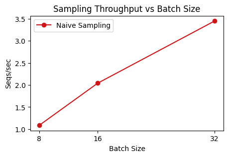
Let’s immediately profile this. For the purposes of RL training, we care more about total throughput than latency. We are OK to wait longer per rollout if it results in a larger sequences/second, as anyways we will be alternating inference and training.

plot_sampling_1()

../_images/cebe678521cb0897508bffa5e7324f94b8baa862d42e1f42363c75e66f995d56.png

Let’s immediately profile this. For the purposes of RL training, we care more about total throughput than latency. We are OK to wait longer per rollout if it results in a larger sequences/second, as anyways we will be alternating inference and training.

There’s a clear trend – larger batchsizes are more efficient. The high-level reason for this is that inference workloads are often bottlenecked by communication. GPUs and TPUs are great at doing large matrix-multiplications, but in inference workloads, we are only processing one token at a time. This means that most of the time in the forward pass is spent communicating data between high-bandwith memory (HBM), which is what is often referred to when saying “a v4 machine has 32GB of memory”, and VMEM, the small buffer (128 MiB) where computation actually takes place.

If we can increase the total batch size we are using, we can improve our sampling throughput. Let’s profile the memory usage of our program. Our first profiling tool is to print the memory usage.

JAX gives us two inline tools to peek at memory usage. At any point in our program, we can call:

def get_memory_usage():
    stats = jax.local_devices()[0].memory_stats()
    return stats['bytes_in_use'] / (1024**3)

to get the per-device usage. Recall that a v4 TPU has 32GB of memory per device. As an example, we can check how much memory our model state takes via:

print(get_memory_usage()) # 7e-05 GB
train_state = jax.jit(init_fn)(params=p)
jax.block_until_ready(train_state) # JAX runs asyncronously.
print(get_memory_usage()) # 1.90 GB

So, we know that around 2 GB is taken up by parameters. We can examine how much memory our sampling call uses using the following JAX helper:

compiled_step = model_apply.lower(params, prompt_tokens[:, :-1], cache=cache).compile()
compiled_stats = compiled_step.memory_analysis()
total = compiled_stats.temp_size_in_bytes + compiled_stats.argument_size_in_bytes \
    + compiled_stats.output_size_in_bytes - compiled_stats.alias_size_in_bytes
print(f"Temp size: {compiled_stats.temp_size_in_bytes / (1024**3):.2f} GB")
print(f"Argument size: {compiled_stats.argument_size_in_bytes / (1024**3):.2f} GB")
print(f"Output size: {compiled_stats.output_size_in_bytes / (1024**3):.2f} GB")
print(f"Total size: {total / (1024**3):.2f} GB")

# === Naive Baseline ====
# Temp size: 0.63 GB
# Argument size: 9.22 GB
# Output size: 8.75 GB
# Total size: 18.60 GB

The sampling step takes 18 GB, when using a per-device batchsize of 32 sequences. In this case, we can easily identify the culprit – it’s the KV cache. Note how the “argument” size of the function is 9 GB. We know that the parameters accounts for only 2 GB, and the prompt tokens are small as they are integers, so the majority of this buffer is the KV cache.

We can also do some napkin math to show why this is reasonable. The Qwen3-1.7B model has 28 layers, 8 KV heads, and a head dimension of 128. For a batch of 32 sequences, each of length 1024:

\[(\underbrace{32}_{\text{batch}} * \underbrace{1024}_{\text{seqlen}} * \underbrace{28}_{\text{layers}} * \underbrace{8}_{\text{KV heads}} * \underbrace{128}_{\text{head dim}} * \underbrace{2}_{\text{K + V}} * \underbrace{4}_{\text{Bytes/fp32}}) = 7.5 \; \text{GB}\]

BF16 Cache#

A quick win is to keep the KV cache in bf16 instead of fp32. This immediately reduces the memory requirement by half, as each bf16 value requires only 2 bytes rather than 4. Indeed, this reduces our requirements:

k = [jnp.zeros((batch_size, max_seq_len, kv_heads, head_dim), 
    dtype=jnp.bfloat16) for _ in range(num_layers)]

# === With bf16 cache ====
# Temp size: 0.64 GB
# Argument size: 4.85 GB
# Output size: 4.38 GB
# Total size: 9.87 GB

Re-using the cache buffer#

It should stand out as odd that we need to pay the memory cost of the KV cache twice. This is a natural consequence of the way that JIT compiles a program, as it allocates a buffer in memory for both the arguments and the output, both of which contain the cache. One approach to this would be to modify our training loop such that only a delta to the cache is outputted, and we splice that together with the full cache in a separate function. But in our case, there is a simple trick that handles this for us. JAX implements a donate_argnums property when compiling functions with JIT, which allows the compiler to reuse an argument buffer for the output. By setting this flag, we can avoid the double-counting of the cache:

@partial(jax.jit, out_shardings=(data_sharding, data_sharding), donate_argnums=2)
def model_apply(params, tokens, cache, key=None):
    ...

# === With buffer reuse ====
# Temp size: 0.64 GB
# Argument size: 4.85 GB
# Output size: 4.38 GB
# Total size: 5.48 GB

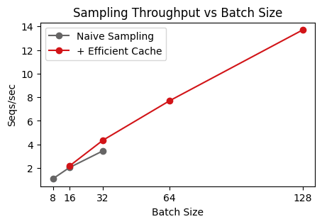
Nice, we’ve reduced our memory requirement down to 25% of the original, from 20 GB to 5 GB! Re-running the original sweep, we can achieve much higher throughput as we can run at a per-device batch of 128.

plot_sampling_2()

../_images/a4b9d69ea84b2307245179acd01c71c2f0d78d2d13a6b927e4d0158cc8d63778.png

Removing all-gathers#

So far, we’ve focused on increasing batch size, without concern for the per-step timings. Indeed, as shown in the curves above, the wallclock time per step is not bottlenecked by FLOPs, but by some other batch-invariant factor.

We can take a closer look using the JAX profiler. We can profile JAX code using:

with jax.profiler.trace('/mount/code/dqlm/lmpo/tensorboard'):
   ...

which then saves a trace to that directory. To read the trace, we can load it into Tensorboard. My preferred way of doing this is to install the Tensorboard plugin in VSCode. You will also need to pip install tensorboard-plugin-profile, otherwise Tensorboard will only show a “no data” screen. Finally, in my setup, I needed to view the trace from the machine it was collected on – it did not work to open the trace on my development machine. This took a while to debug so I hope you won’t have to go through it.

rl-infra-fig2

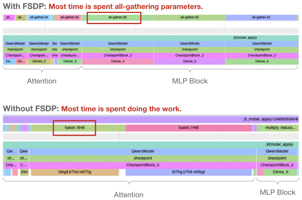
To the careful reader, our issue should stand out. Naively, our model was sharded using FSDP, which distributed parameters among devices. Every iteration, the devices would perform an all-gather to materialize the full weights for the layer. This is good for training, where we’re operating over large batches, but it’s a dealbreaker in inference. Instead, we can make our sampling much faster by performing a single all-gather at the start of the sampling procedure, and keeping them replicated on each device until the sampling loop has finished. This comes at a cost – we need to allocate around 9 GB to keep the full parameters – but it’s more than worth it for the speed boost.

plot_sampling_3()

../_images/db1f0f8e78f51690b8c75256b71652b68d8d6190410906b726174c1a409349e9.png

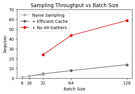
Comparing with vLLM. We can sanity check the efficiency of our system by comparing the speeds to off-the-shelf inference engine like vLLM. When profiling vLLM with vllm bench throughput --input-len 256 --output-len 1024 --model Qwen/Qwen3-1.7B --max-model-len 2048 --num-prompts 2048, we get a rough throughput of 0.5 seconds per sequence. In comparison, our LMPO engine requires an average of around 0.08 seconds per sequence, a roughly 5x speedup:

Method	Sequences/sec on v4-8
vLLM	\(\sim 2 \)
LMPO (Naive)	\(\sim 0.8 \)
LMPO (Optimized)	\(\sim 12 \)

It is nice to know that we are in the right ballpark for performance, even when compared against battle-tested implementations. For reference, our optimized LMPO implementation was able to utilize a per-device batch of 128, whereas vLLM used a per-device batch of 64.

Further improvements. We did not cover all possible optimizations to the sampling pipeline. Some common techniques are:

If the model is too large to fit on a single device, we can use tensor parallelism. This is much preferred over FSDP, as the devices can communicate the activations (which are small for inference) rather than the parameters.
Dynamic cache sizing. Here, we’re calculating attention over the entire sequence length at each step, even though the cache is mostly zeros. We could improve this by compiling a separate graph for each power-of-two sequence length, and only using the amount we need at each step.
Lower precision. We’re using bfloat16, but it may be fine even use fp8.

Part 2: Training#

Alright, it’s now time to examine the training loop. Remember that the adjustments above (removing FSDP, KV cache usage) are for the inference setting, so we won’t be inheriting them for training. Our baseline here is the same basic implementation of the Qwen3-1.7B model, trained via FSDP. Our main activations are in bfloat16, and attention and RMSNorm are calculated in fp32.

plot_sampling_4()

../_images/14d362b4bf7e0599455506d243a31ef3ec2e7f588c824d92877fcd2add9787b3.png

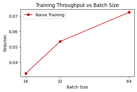
For a sequence length of 1024, we’re able to reach a global batchsize of 64 before running out of memory. This is a total batch of 65K tokens. Remember that we are training on a cluster of 16 devices, so this approximately 4000 tokens per device. This is a pretty healthy per-device batch, and it’s enough for us to be compute-bound on dense layers, i.e. we can expected our TPU FLOPs utilization to be quite high. However, there may still be overhead for operations such as all-gathering the parameters and calculating attention.

If we want to train on longer sequence lengths, like 8192 as is common for reasoning models, we’ll see that we quickly run out of memory, even with only a single sequence per device (note this is still 8192 tokens, which is still a decent batch size in practice).

Our next immediate goal is to see if we can decrease our memory requirements, therefore allowing us to increase batch size and sequence length. We’ll get a good sense of memory consumption by utilizing the JAX profiler again. This time, we’re focusing on the “Memory Profiling” tab. In this tab, we can examine the memory usage of JIT-compiled functions. Make sure to select ‘update’ from the left tab.

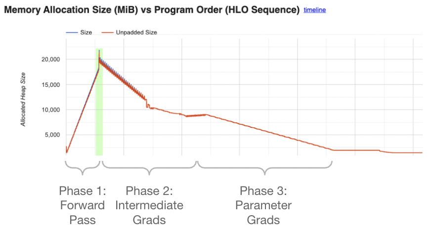
We see here a typical pattern for a calculating a gradient. First, we perform a forwards pass on the model, keeping intermediate activations in memory. Next, we start on the backwards passing, calculating the intermediate gradients with respect to each activation. Finally, we take the gradient with respect to the parameters themselves, which will return the gradient. We can explicitly write down these stages for a simple two-layer MLP:

def manual_grad(params, data_input, data_output):
    W1, b1, W2 = params

    # Phase 1: Forward Pass.
    h1 = W1 @ data_input
    h2 = h1 + b1[:, None]
    h3 = h2 * (h2 > 0)
    h4 = W2 @ h3
    loss = jnp.mean(jnp.square(h4 - data_output))

    # Phase 2: Backward Pass, calculate interemediate gradients.
    d_h4 = 2 * (h4 - data_output) / data_output.shape[1]
    d_h3 = W2.T @ d_h4
    d_h2 = d_h3 * (h2 > 0)
    d_h1 = d_h2

    # Phase 3: Backward Pass, calculate parameter gradients.
    d_W2 = d_h4 @ h3.T
    d_b1 = jnp.mean(d_h2, axis=1)
    d_W1 = d_h1 @ data_input.T

    return [d_W1, d_b1, d_W2], loss

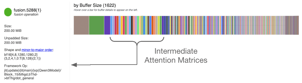
We can examine the specific shapes of each operation to see which operations are taking the most memory. One shape in particular stands out for transformers – there is a (batch, attn_heads, 1280, 1280) matrix, in fact there are 28 of them. This is the attention matrix, and it’s quite large. Even worse, this scales with our sequence length squared, so it’s a problem if we want to train on longer sequences. JAX even tells us exactly where we’re computing this, hinting at the problem:

qk = jnp.einsum("bthgd,bThd->btThg", q, k)

Flash Attention#

Thankfully, we can use flash attention to avoid saving this matrix. In the flash attention algorithm, we never form an explicit (seqlen, seqlen) attention matrix, and instead compute the softmax-weighted output on-the-fly, in chunks. The main benefit of this is for speed – moving a large attention matrix to and from the HBM to VMEM is an expensive communication operation. However, the second benefit is that this allows us to forgo saving the attention matrix for use in the backwards pass. Instead, we’ll compute the backwards gradient using a similar chunked calculation.

For our setting, we’ll make use of the Pallas flash attention implementation built into JAX. We can replace our manual einsum implementation with a kernel call. Note that we need to wrap the call in shard_map, which explicitly tells the JAX compiler how computation should be split among devices. In the case of data-parallelism, this is quite simple, as each device can just process its own batch of sequences.

@jax.shard_map
def flash_attention(q, k, v, token_mask):
    k, v = repeat_kv_heads(k, v, q.shape[2] // k.shape[2])
    segment_ids = SegmentIds(token_mask, token_mask)
              
    return pallas_flash_attention_tpu(
        q.transpose(0, 2, 1, 3),
        k.transpose(0, 2, 1, 3),
        v.transpose(0, 2, 1, 3),
        sm_scale=1.0 / q.shape[-1]**0.5,
        block_sizes=block_sizes,
        causal=True if k.shape[1] == q.shape[1] else False,
        segment_ids=segment_ids,
    ).transpose(0, 2, 1, 3).astype(jnp.bfloat16)

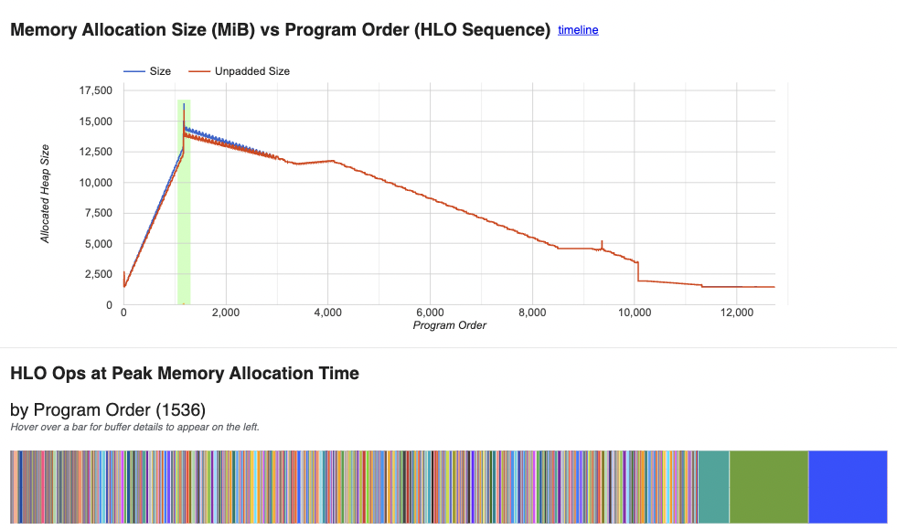
Looking at the memory profiler now, we can see that our total requirements have gone down from 20GB to 15GB. Looking at the buffer list, all the attention matices are now gone.

Gradient Rematerialization#

However, we’re still saving a lot of intermediate activations during the forwards pass. We can reduce this requirement even further using gradient rematerialization, also referred to as activation checkpointing or gradient checkpointing. The basic idea is that instead of saving every intermediate activation, we can just save activations at specific points, then re-compute the inbetween values later. A typical strategy is to only save the input to each transformer block, which is a small matrix of size (batch, seqlen, 2048) for our model – note that this avoids saving the intermediate MLP activations, where are (batch, seqlen, 6144).

In JAX, we can tell the compiler to utilize gradient rematerialization by wrapping a function with @jax.remat. We can also wrap a Flax module with nn.remat, which is what we will do to our entire Block module above.

BlockFn =  nn.remat(Block)

Let’s take a look at the profiler once more.

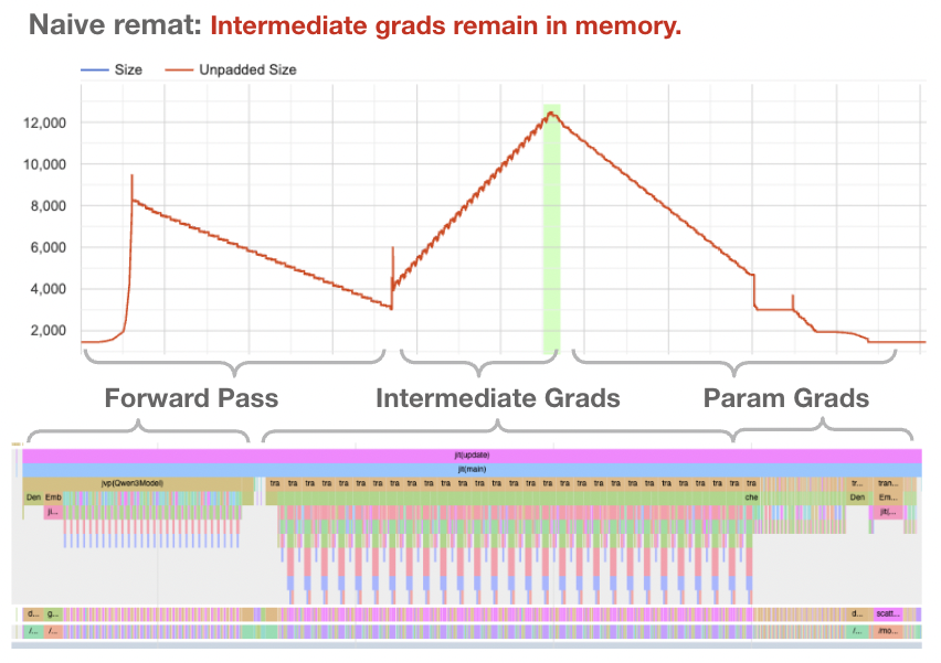
Indeed, our forward pass now requires significantly less memory. But, the backwards pass as a whole is still requiring quite a large amount of memory. What’s the big deal?

First, let’s be clear about why the above memory graph is unsatisfying – even through we are not saving intermediate buffers during the forwards pass, we are saving these buffers for the entire backwards pass, and not freeing them after each layer.

Consider the gradient to an activation at layer 5. This gradient is needed for 2 uses – to calculate the gradient for the layer 4 activation, and to calculate the gradient for the parameters of layer 5. To limit our memory usage, we would like to perform both of these calculations, then delete the intermediate gradient. In other words, we want to interleave phases 2 and 3. But if we look at what the JAX compiler is doing, it is instead calculating all the phase 2 intermediates, and only afterwards consuming them for phase 3.

Magic XLA Flag#

Unfortunately, this is the limit of where I know how to debug. JAX compiles the written Python programs into XLA via its internal compiler, and it is an opaque process (at least to me.) If anyone has a real answer for how to force JAX to interleave these phases, please let me know! That said, I did end up finding a magical XLA flag that seems to achieve the desired outcome:

os.environ['LIBTPU_INIT_ARGS'] = '--xla_tpu_enable_latency_hiding_scheduler=false`

This flag disables the “latency hiding scheduler” that attempts to overlap communication and computation. My best understanding is that for some reason, JAX is delaying the phase 3 calculations due to the communication needed to all-reduce the gradients for FSDP. In fact, if we disable FSDP, then we can avoid the problems entirely, and JAX will compile a program that correctly interleaves phase 2 and phase 3. Unfortunately, we do need FSDP to train models of any reasonable size. This flag is the best solution I could find, although, I’m not sure if there will be unintentional consequences…

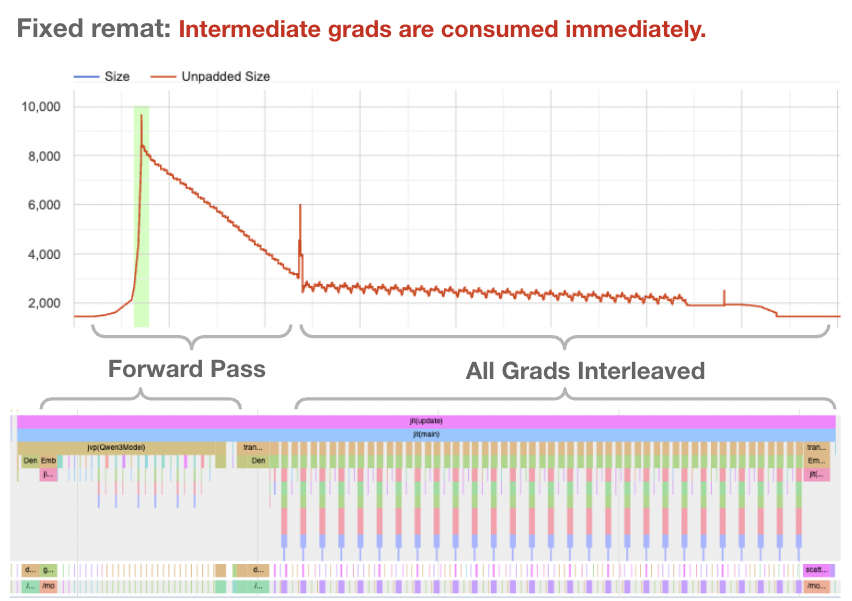
Nice! This time, we’re able to bring our memory footprint down to 9 GB, and if we look at the trace viewer, we can see that phases 2 and 3 are correctly interleaved.

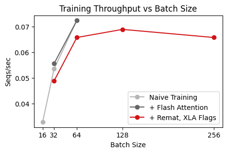
Finally, let’s benchmark our new improved training pass. With the changes above, we are able to support a global batch size of 256, which is 4x the previous batch size! Also, we’re able to train on sequence lengths of 8192, and we can even do so at a batchsize of 32. However, it’s worth noting that using remat does come at a cost, as we need to re-calculate intermediate values.

plot_sampling_5()

../_images/25c3cceb8a17cbb39195756e6e9212405c04f169bc3c2e0df6536d7886146342.png

Conclusion#

With the changes above, I’m pretty happy with the speed of our RL loop. As these kinds of optimizations are always a rabbit hole, I’m going to call it here.

The three profiling techniques I found quite useful are to:

Print the overall memory usage with jax.local_devices()[0].memory_stats(). This is essentially free to do, but you’ll only get a sense of total memory usage.
Use compiled_step.memory_analysis() to see the memory requirements for a JIT-compiled function. This is helpful to determine if you’re wasting memory on the input/output buffers.
When using jax.remat, you can use jax.ad_checkpoint.print_saved_residuals to print which intermediate arrays JAX might try to save during the forwards pass. However, note that these arrays are printed before compilation, and in practice, the compiler will usually remove most these.
If the problem is deep, use the profiler. jax.profiler.trace is a great tool. Use the trace viewer to figure out what your program is actually running, and use the memory viewer to see what’s causing OOM issues. There are other tabs too, but I found these two the most helpful.

You can check out the full codebase, including the actual code, at kvfrans/lmpo.