Variational Auto-Encoders

Variational Auto-Encoders#

The variational auto-encoder learns to compress data, and in doing so can generate new data.

The first breakthroughs in deep learning focused on classification. However, classification objectives needed labelled datasets, which were expensive to curate. The question arose – what can we learn from just unlabelled data? A solid answer is to learn a generative model – neural networks that directly model the data they are trained on, and can generate new samples.

A classic generative modelling setting is that of image generation. We have a dataset of unlablled images, and we would like to train a neural network that, when queried, can generate images that match this dataset. Image and video generative models are what power many popular models such as Stable Diffusion, Midjourney, Sora, etc.

from jaxtransformer.utils.datasets import get_dataset

dataset = get_dataset('celebahq64', 64, is_train=True) # Normalized to [-1, 1].
dataset_valid = get_dataset('celebahq64', 64, is_train=False) # Normalized to [-1, 1].
plot_dataset(dataset)

../_images/58f660bd03b6a5e3f1d5368ff56fc20263a4527818fa2ef7f73d2b13c245ad6a.png

Fig: Samples from the CelebAHQ dataset.

Latent Variable Models#

In the generative modelling setting, we would like to train a network which mimics the data distribution. As the ground-truth distributions can be arbitrarily complex, a common technique is to employ latent variable models, which factor the distribution into an unobserved latent variable, along with a mapping from latents to data points. A latent variable takes the following form:

\[ p(x) = \int_z p(x|z) p(z) \]

where \(x\) represents a data point, and \(z\) represents the latent variable.

While latent variables are not directly visible, they can be inferred from other observations. In our CelebA dataset, we only have access to the raw images. However, we know that faces that generally be described in terms of features such and hair color, eye shape, and so on. When we can represent data points using a dense vector of features, we call that vector a latent representation of the data point.

The Noise-Conditioned Generator#

In an arbitrary latent variable model, both the prior \(p(z)\) and the conditional \(p(x|z)\) can be learned. For ease of training, it is common to only learn the conditional function, and set the prior to a simple random distribution, such as a Gaussian. This setup is known as the noise-conditioned generator, and it allows us to frame generative models as neural networks of the form \(p_\theta(x|z)\), where \(z \sim N(0,1)\). To generate samples from a noise-conditioned generator, we can simply sample a random \(z\) vector, then pass it through the generator network.

Importantly, using a noise-conditioned generator allows the conditional \(p(x|z)\) to be a simple distribution (i.e. Gaussian, or even a determinstic function), while the full \(\int p(x|z)p(z)\) distribution can remain expressive.

Noise-conditioned generators are a common form in many modern generative models, such as the variational auto-encoder, generative adversarial networks, and diffusion models. In each setting, there is a different objective used to train the generator network. We will focus this time on the variational auto-encoder, which uses a simple probabilistic objective.

vae

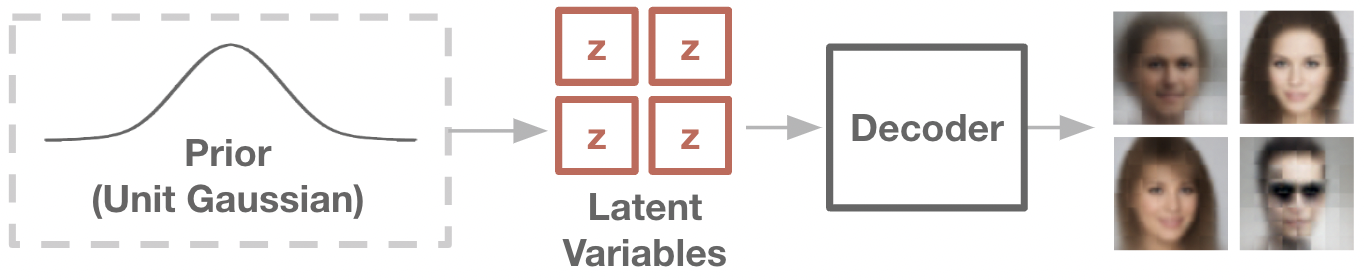
Fig: Noise-conditioned generators learn a neural network to transform noise into generated samples.

Variational Auto-Encoders#

The core problem in latent variable modelling is that the latent variables are never observed, so the mapping \(p(x|z)\) is not defined by the data. One straightforward method of discovering such a mapping is the autoencoder. An autoencoder consists of two networks – an encoder, which maps an image to a latent variable, and a decoder, which plays the role of the generator and maps the latent variable back to the image.

To train an autoencoder, we can jointly train the encoder and decoder towards minimizing a reconstruction objective, often a standard mean-squared-error over pixels. Given an image from the dataset, the encoder should form a latent representation, with which the decoder than then recover the original image. This is equivalent to maximizing the likelihood of the data under the encoder-decoder model.

In most cases, we set the dimensionality of the latent vector to be considerably smaller than the raw input. For example, an image may be 32x32x3 pixels, but its corresponding latent representation may be a 16-dimensional vector. In this way, autoencoders are often seen as learning to compress data into a denser form (along with decompressing it back).

A standard autoencoder is not a generative model. While we do have a mapping between latents and data points, we don’t have any way to sample new latents (and therefore generate new samples). The variational auto-encoder (VAE) will develop this capability, giving us our first generative model.

The key is that the VAE also includes a specific constraint: the distribution of encoded latent variables should match a simple prior distribution, often the unit Gaussian. If this constraint is satisfied along with the reconstruction objective, then the decoder portion of the VAE is precisely the noise-conditioned generator we desire. We can generate novel samples, simply by querying this decoder with random Gaussian noise.

Concretely, we will view the encoder \(q_\theta(z|x)\) and decoder \(p_\theta(x|z)\) as neural networks which output the mean and variance of a Gaussian distribution. As our reconstruction objective, we aim to maximize the log-likelihood of the data, when passed through the encoder and decoder. And as a prior-matching objective, we aim to minimize the KL divergence between the encoder distribution and the unit Gaussian. Thus, the full VAE objective can be written as:

\[L(\theta, x) = \underbrace{E_{z \sim q_\theta(z|x)}[\log p_\theta(x|z)]}_{\text{Reconstruction Objective}} + \underbrace{KL(q_\theta(z|x) || q(z))}_{\text{Prior-Matching Objective}}\]

where \(q(z)\) is an uninformative prior, often the unit Gaussian.

vae

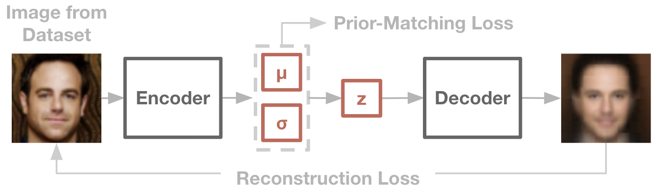
Fig: The VAE training objective is to recreate the original data point, while matching the encoder’s distribution to that of a Gaussian prior.

Implementation: VAE on CelebAHQ#

We’re almost ready to implement a simple VAE. First, let’s go over a few analytical properties of the Gaussian, so we can translate them into code.

For the reconstruction objective, note that the log-likelihood of a point \(x\) under a Gaussian parameterized by mean \(\mu\) and standard deviation \(\sigma\) is:

\[ - \log p(x) = \log(2 \pi) + \log(\sigma) + \frac{(x - \mu)^2}{2 \sigma^2}. \]

where the constant \(\log(2 \pi)\) term can be dropped during optimization.

def reconstruction_loss(x, mean, log_std):
   return log_std + jnp.square((x-mean)/jnp.exp(log_std))

If this looks suspiciously like the mean-squred error loss, you are on the right track. MSE loss is often justified as maximzing the log-probability of a datapoint under a Gaussian with unit variance.

For the prior matching objective, we would like to minimize the KL divergence between q(z|x) and the unit Gaussian q(x). Remember that q(z|x) is also a Gaussian, parametermized by mean and variance. Thankfully, there’s a simple analytical form to this objective we can arrive at. For now, we will just take it for granted – there will be a proper derivation in a later section.

def prior_matching_loss(mean, log_std):
    return jnp.exp(log_std) + jnp.square(mean) - 1 - log_std

With those key equations in mind, let’s implement our VAE. We’ll again use our jaxtransformer library to define a transformer backbone for the encoder and decoder models. We will process images using a patch embedding, and use an embedding token to represent the final output of the encoder.

from jaxtransformer.transformer import TransformerBackbone
from jaxtransformer.modalities import PatchEmbed, PatchOutput, get_2d_sincos_pos_embed
from jaxtransformer.utils.train_state import TrainState

class Encoder(nn.Module):
    hidden_size: int
    z_dim: int
    patch_size: int
    num_patches: int

    @nn.compact
    def __call__(self, x):
        x = PatchEmbed(patch_size=self.patch_size, hidden_size=self.hidden_size)(x)
        x = x + get_2d_sincos_pos_embed(None, self.hidden_size, self.num_patches)
        embed_token = nn.Embed(num_embeddings=1, features=self.hidden_size)(jnp.zeros((x.shape[0], 1), dtype=jnp.int32))
        x = jnp.concatenate([embed_token, x], axis=1)
        x = TransformerBackbone(depth=4, num_heads=4, hidden_size=self.hidden_size, 
            use_conditioning=False, use_causal_masking=False, mlp_ratio=4)(x)
        x = nn.LayerNorm()(x)
        x = nn.Dense(features=self.z_dim * 2)(x[:, 0, :])
        mean, log_std = jnp.split(x, 2, axis=-1)
        return mean, log_std
    
class Decoder(nn.Module):
    hidden_size: int
    patch_size: int
    num_patches: int
    channels_out: int

    @nn.compact
    def __call__(self, z):
        x = nn.Dense(features=self.hidden_size)(z)
        x = jnp.tile(x[:, None, :], (1, self.num_patches, 1))
        x = x + get_2d_sincos_pos_embed(None, self.hidden_size, self.num_patches)
        x = TransformerBackbone(depth=4, num_heads=4, hidden_size=self.hidden_size, 
            use_conditioning=False, use_causal_masking=False, mlp_ratio=4)(x)
        x = nn.LayerNorm()(x)
        x = PatchOutput(patch_size=self.patch_size, channels=self.channels_out*2)(x)
        mean, log_std = jnp.split(x, 2, axis=-1)
        return mean, log_std

class VAE(nn.Module):
    hidden_size: int = 256
    z_dim: int = 64
    patch_size: int = 8
    input_side_len: int = 64
    input_channels: int = 3

    def setup(self):
        num_patches = (self.input_side_len // self.patch_size)**2
        self.encoder = Encoder(self.hidden_size, self.z_dim, self.patch_size, num_patches)
        self.decoder = Decoder(self.hidden_size, self.patch_size, num_patches, self.input_channels)

    def __call__(self, x, rng):
        z_mean, z_log_std = self.encoder(x)
        noise = jax.random.normal(rng, z_mean.shape)
        z = z_mean + jnp.exp(z_log_std) * noise
        x_mean, x_log_std = self.decoder(z)
        return x_mean, x_log_std, z_mean, z_log_std
    
    def encode(self, x):
        return self.encoder(x)[0]
    
    def decode(self, z):
        return self.decoder(z)[0]

@jax.jit
def loss_fn(params, x, rng):
    x_mean, x_log_std, z_mean, z_log_std = VAE().apply({'params': params}, x, rng)
    reconstruction_loss = 0.5 * jnp.mean(jnp.sum(((x - x_mean)/jnp.exp(x_log_std))**2 + x_log_std, axis=(1,2,3)))
    kl_loss = 0.5 * jnp.mean(jnp.sum(jnp.exp(z_log_std) + z_mean**2 - 1 - z_log_std, axis=-1)) * 100
    info = {'reconstruction_loss': reconstruction_loss, 'kl_loss': kl_loss, 'avg_x_std': jnp.mean(jnp.exp(x_log_std)), 'avg_z_std': jnp.mean(jnp.exp(z_log_std))}
    return reconstruction_loss + kl_loss, info

Let’s let our model train, and look at the results:

plot(losses, reconstruction_losses, kl_losses, valid_losses, x_std, z_std)

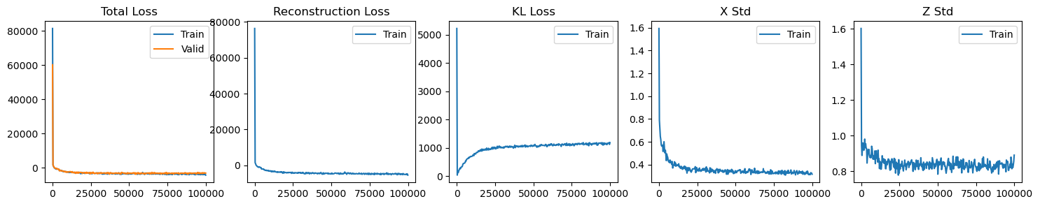
../_images/9aae1a9734de3fdd865ae98bba8c837454b20e2d7808de6e39dd3fde91344fe9.png

Notice the tradeoff between reconstruction loss and the prior-matching loss. Training a VAE is a balancing act – we want to encode information into the latent variable which is helpful for reconstruction, yet the prior-matching loss penalizes information.

We can also see the standard deviation of our decoder decrease over time, which is a good sanity check. A lower standard deviation means the decoder is more confident about the images it produces, i.e. the reconstructions will be less blurry.

Now, let’s examine some reconstructions. We will sample some ground-truth images from our dataset, encode them, then decode them back out.

true_images, _ = next(dataset)
z = model.apply({'params': train_state.params}, true_images, method=model.encode)
reconstruction = model.apply({'params': train_state.params}, z, method=model.decode)
plot_reconstruction(true_images, reconstruction)

Reconstruction error: 0.025968783

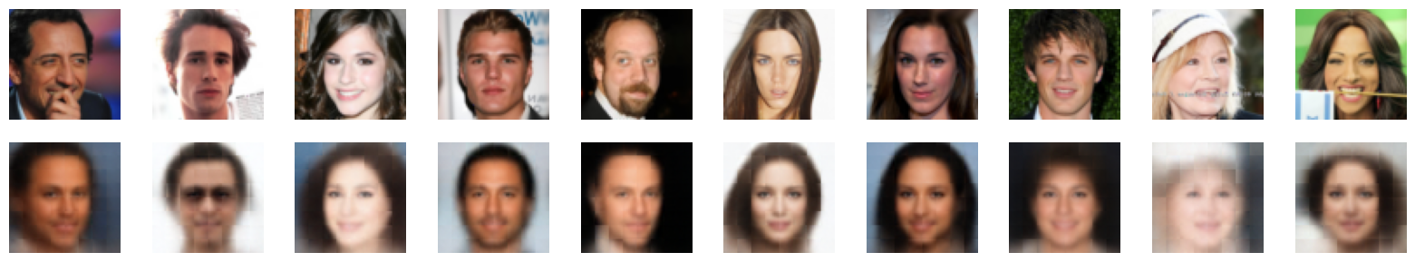
../_images/9aafc0bbfb5bcde8aeb21aeb73e1490e2c7972b9fd7dda66dc1106f8b2877cac.png

Not bad! The general features of each image are preserved in the recreation.

We can now sample novel generations, by sampling noise vectors, and passing these noise vectors into the decoder.

# Sample noise, then decode.
z = jax.random.normal(jax.random.PRNGKey(0), (10, 64))
img = model.apply({'params': train_state.params}, z, method=model.decode)

# Plot.
img = (np.array(img).astype(np.float32) + 1) / 2
img = np.clip(img, 0, 1)
fig, axs = plt.subplots(1, 10, figsize=(20, 5))
for i, ax in enumerate(axs):
    ax.imshow(img[i], cmap='gray')
    ax.axis('off')

../_images/db24d25275b18777c8a31fe3aba86ae82204d1e59b1b38d4a713e1bdb89328b8.png

You’ll notice that in both reconstruction and generation, the outputs are quite blurry. Blurriness is a consistent weakness of VAE generations. The reason for this is twofold:

First, the prior-matching term in the VAE encourages each latent variable to contain as little information as possible. This means that there will always be some uncertainty about the original image, even when given its matching latent representation.
Second, we parameterize the decoder as a Gaussian distribution. Gaussian distributions maximize log-likelihood by matching the mean of a distribution. If the ground-truth pixels take on a bimodal distribution of 0 or 1, a Gaussian will predict the mean of 0.5. For images in pixel space, this results in blurriness. Uncertainty in pixel space results in blurry generation.

Interpolating in Latent Space#

A well-trained VAE learns a latent representation that maximally compresses the information in an image. Because of this, the structure of the latent space is much tighter than that of the original pixel space. If we interpolate between two images in pixel space, the midpoints have little semantic meaning. However, the same interpolation in latent space can yield meaningful images.

true_images, _ = next(dataset)
interp = np.linspace(0, 1, 10)

# Image-Space Interpolation.
image_interp = true_images[0] * interp[:, None, None, None] + true_images[1] * (1 - interp[:, None, None, None])
img = (np.array(image_interp).astype(np.float32) + 1) / 2
img = np.clip(img, 0, 1)
fig, axs = plt.subplots(1, 10, figsize=(20, 5))
for i, ax in enumerate(axs):
    ax.imshow(img[i], cmap='gray')
    ax.axis('off')

# Latent-Space Interpolation.
z = model.apply({'params': train_state.params}, true_images[:2], method=model.encode)
z_interp = z[0] * interp[:, None] + z[1] * np.sqrt(1 - interp[:, None]**2)
reconstruction = model.apply({'params': train_state.params}, z_interp, method=model.decode)
img = (np.array(reconstruction).astype(np.float32) + 1) / 2
img = np.clip(img, 0, 1)
fig, axs = plt.subplots(1, 10, figsize=(20, 5))
for i, ax in enumerate(axs):
    ax.imshow(img[i], cmap='gray')
    ax.axis('off')

../_images/13cc1c20eb80935ca10940ba2038c5b549578f3d4c945ac95035f14a9df521d5.png

../_images/571738e4642661799f4dc219fc2b0f66fc58a5d0df85850d413cc88c5438e68e.png

Derivation of VAE from Evidence Lower Bound (ELBO)#

The VAE objective has a principled derivation, which stems from maximizing a lower bound on the log-likelihood of the dataset. We skipped over this derivation in favor of a more intuitive justification in the previous section. Now, we will go over the full derivation.

First, the overall goal in any generative modelling problem is to learn a distribution which maximizes the log-likelihood of the dataset.

\[ L(\theta) = \sum_{x \sim D} \log p(x) \]

Unfortunately, we don’t have a way to calculate \(p(x)\). Remember that our generator is of the form \(p_\theta(x|z)\), i.e. conditional on the latent variables. Some may ask, can we use the following relation:

\[ \log p(x) = \log \int_z p_\theta(x|z)p(z) dz \]

but, the integral here is over all possible \(z\) values, and hence intractable to compute. By Bayes’ rule, the “true” latent distribution of \(p(z|x)\) is also intractable.

Instead, we will rely on an approximation of \(p(z|x)\) – our decoder network \(q_\theta(z|x)\). Introducing this term into our equation for \(\log p(x)\):

\[\begin{split} \begin{align} \log p(x) &= \log \frac{p_\theta(x|z)p(z)}{p(z|x)} \\ &= E_{q} \left[ \log \frac{p_\theta(x|z)p(z)}{p(z|x)} \right] \\ & = E_{q} \left[ \log \frac{p_\theta(x|z)p(z)}{p(z|x)} \frac{q_\theta(z|x)}{q_\theta(z|x)} \right] \\ & = E_{q} \left[ \log \frac{p_\theta(x|z)p(z)}{q_\theta(z|x)} \frac{q_\theta(z|x)}{p(z|x)} \right] \\ & = E_{q} \left[ \log \frac{p_\theta(x|z)p(z)}{q_\theta(z|x)}\right] + E_{q} \left[ \log \frac{q_\theta(z|x)}{p(z|x)} \right] \\ & = \underbrace{E_{q} \left[ \log \frac{p_\theta(x|z)p(z)}{q_\theta(z|x)}\right]}_{\text{ELBO}} + \underbrace{KL(q_\theta(z|x) || p(z|x))}_{\text{Intractable KL}} \\ \end{align} \end{split}\]

We now have a term commonly referred to as the evidence lower bound (ELBO). The remaining term is a KL divergence between \(q_\theta(z|x)\) and \(p(z|x)\), and since the latter is intractable, we are unable to calculate this term in practice. That said, KL divergences are strictly positive, so the ELBO is a lower bound on \(\log p(x)\).

The ELBO term ends up being exactly what we optimize for in the VAE objective. To see this, we will break the ELBO into two familiar parts:

\[\begin{split} \begin{align} \text{ELBO} &= E_{q} \left[ \log \frac{p_\theta(x|z)p(z)}{q_\theta(z|x)}\right] \\ &= E_{q} \left[ \log p_\theta(x|z) \frac{p(z)}{q_\theta(z|x)}\right] \\ &= E_{q} \left[ \log p_\theta(x|z) + \log \frac{p(z)}{q_\theta(z|x)}\right] \\ &= E_{q} \left[ \log p_\theta(x|z) \right] + E_{q} \left[ \log \frac{p(z)}{q_\theta(z|x)}\right] \\ &= \underbrace{E_{q} \left[ \log p_\theta(x|z) \right]}_{\text{Reconstruction Objective}} - \underbrace{KL(q_\theta(z|x) || p(z))}_{\text{Prior-Matching Objective}} \\ \end{align} \end{split}\]

And this is the VAE objective. For more details on the ELBO derivation, see: https://mpatacchiola.github.io/blog/2021/01/25/intro-variational-inference.html

Derivation of Analytical KL Loss#

For arbitrary probabiltiy distributions, measuring the KL divergence involves either an intractable integral, or approximating the KL with many samples. However for certain distributions, notably Gaussians, the true KL divergence can be computed analytically. This technique is used to derive the KL regularization loss in the VAE. We wish to calculate the KL divergence between a Gaussian q(z|x) and the unit Gaussian p(z).

Starting from the definition of KL divergence:

\[\begin{split} \begin{align} KL & = E_q[ \log q(z|x) - \log p(z)] \\ & = E_q[ -\log(2 \pi) - \log(\sigma) - \frac{(z - \mu)^2}{2 \sigma^2} - \log p(z)] \qquad \text{(Log-prob of Gaussian.)} \\ & = E_q[ -\log(2 \pi) - \log(\sigma) - \frac{(z - \mu)^2}{2 \sigma^2} + \log(2 \pi) - \frac{z^2}{2}] \qquad \text{(Log-prob of unit Gaussian.)} \\ & = \underbrace{E_q[ - \log(2 \pi) - \log(\sigma) + \log(2 \pi)]}_{\text{Expectation 1}} + \underbrace{E_q \left[ - \frac{(z - \mu)^2}{2 \sigma^2} \right] }_{\text{Expectation 2}} + \underbrace{E_q \left[ - \frac{z^2}{2} \right]}_{\text{Expectation 3}} \end{align} \end{split}\]

Let’s deal with each of these three expectation terms one-by one. For the first expectation, there are no z terms, so we can drop the expectation entirely.

\[ E_q[ - \log(2 \pi) - \log(\sigma) + \log(2 \pi)] = E_q[-\log(\sigma)] = -\log(\sigma) = -(1/2) \log (\sigma^2) \]

For the second expectation, we make use of the fact that for a Gaussian, \(E_q[(z-\mu)^2] = \sigma^2\) (variance).

\[ E_q \left[ -\frac{(z - \mu)^2}{2 \sigma^2} \right] = -\frac{\sigma^2}{2 \sigma^2} = -(1/2) \]

For the third expecation, we again make use of analytical variance. Remember that \(\sigma^2 = E[z^2] - E[z]^2 = E[z^2] - \mu\).

\[ E_q \left[ - \frac{z^2}{2} \right] = -(1/2) E_q[z^2] = (1/2)(\sigma^2 + \mu^2) \]

Putting the three terms back together, we arrive at the final analytical KL term:

\[ KL(q(z|x) || p(z)) = (1/2) (-\log(\sigma^2) - 1 + \sigma^2 + \mu^2) \]

To sanity check, let’s verify that the minimizer of this loss occurs when \(\mu = 0\) and \(\sigma = 1\).

\[\begin{split} (d/d \mu) [-\log(\sigma^2) - 1 + \sigma^2 + \mu^2] = 2 \mu \qquad \text{Minimum at} \; \mu = 0. \\ (d/d \sigma) [-\log(\sigma^2) - 1 + \sigma^2 + \mu^2] = 2 \sigma - 2/\sigma \qquad \text{Minimum at} \; \sigma = 1. \end{split}\]

Can MSE loss be used for reconstruction loss?#

Yes, with some caveats. Many VAE implementations will just use an MSE loss for the reconstruction term, rather than the Gaussian log-likelihood we use in our implementation. The key intution is that MSE loss is just a special case of the Gaussian log-likelihood, with variance fixed at 1. Learning the variance lets the model make a more accurate prediction, so it’s the more ideal thing to do.

How should the tradeoff between reconsturction and KL be tuned?#

In our VAE implentation, we have a hyperparameter beta that trades off between the reconstruction loss and the prior-matching loss. This hyperparameter is not present in the original VAE derivation. However, note that the relative magnitudes of the reconstruction and prior-matching terms depend on the dimensionality of each space. If we sum over channels vs. taking the mean, for example, our weighting will change. Thus, my current reccomendation is to simply find a good beta term empirically. These concepts are covered in more detail in the Beta-VAE paper.

KL-Regularization is performed elementwise, not batchwise.#

A common misconception of the VAE is that the prior-matching term encourages the global distribution of latent variables to look Gaussian. In other words, a batch of encoded latents should roughly resemble the unit Gaussain. This is a misunderstanding – the prior-matching term encourages eacb indivudual latent variable to look Gaussian, regardless of the other latents in the batch.

Why are VAEs often blurry?#

In the end, the mismatch between pixelwise distance and perceptual distance causes blurriness. In the stnadard VAE formulation, we assume that our decode follows a Gaussian distribution. Gaussian distributions maximize log-likelihood by matching the mean of a distribution. Thus, if a pixel could possible take on the values of 0 or 1, the optimal Gaussian predictor will center around 0.5, resulting in blurriness.

The Reparameterization Trick#

The reparameterization trick is a technique used to backpropagate through the stochastic encoder. Remember that our encoder defines a Gaussian; but the neural network itself is deterministic. To handle this, the reparameterization trick formulates the encoder to output a deterministic mean and variance, which are combined with a randomly sampled Gaussian noise during the forward pass. This gives us a low-variance estimator for the true derivative of the encoder. We sneakily used this trick in the main VAE section. There are other options here, for example, one can use REINFORCE-style updates to take derivatives over the expectation, but the reparameterization trick is the standard for its simplicity and stability.

Variational Auto-Encoders

Contents

Variational Auto-Encoders#

Latent Variable Models#

The Noise-Conditioned Generator#

Variational Auto-Encoders#

Implementation: VAE on CelebAHQ#

Interpolating in Latent Space#

Derivation of VAE from Evidence Lower Bound (ELBO)#

Derivation of Analytical KL Loss#

Can MSE loss be used for reconstruction loss?#

How should the tradeoff between reconsturction and KL be tuned?#

KL-Regularization is performed elementwise, not batchwise.#

Why are VAEs often blurry?#

The Reparameterization Trick#