Activation Functions#
Activation functions are elementwise functions which allow networks to learn nonlinear behavior.
Between dense layers, we place an activation function to transform the features elementwise. They are also known as nonlinearities as the purpose of an activation function is to break the linear relationship defined by the dense layers.
Squashing Activations: Sigmoid, Tanh#
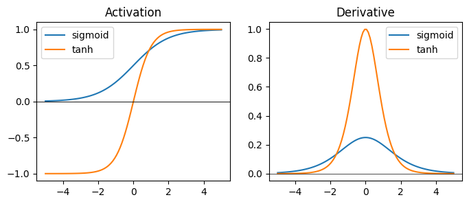
The first activation functions were proposed from a biologically inspired perspective, and aimed to model the ‘spiking’ behavior of biological neurons. The sigmoid function squashes inputs to a range between (0,1), and tanh (hyperbolic tangent) squashes between (1,1). Squashing activations are good for ensuring numerical stability, since we know the magnitude of the outputs will always be constrained. However, when the inputs are too large in magnitude, the gradient of a squashing function will approach zero. This creates the vanishing gradient problem where a neural network will have a hard time improving when features become too large.
def plot_activations(fn_list, fn_names):
    fig, axs = plt.subplots(1, 2, figsize=(8, 3))
    x = jnp.linspace(-5, 5, 100)
    for i in range(len(fn_list)):
        axs[0].plot(x, fn_list[i](x), label=fn_names[i])
        axs[1].plot(x, jax.vmap(jax.grad(fn_list[i]))(x), label=fn_names[i])
    axs[0].axhline(0, color='black', linewidth=0.5)
    axs[0].axhline(0, color='black', linewidth=0.5)
    axs[0].title.set_text('Activation')
    axs[0].legend()
    axs[1].axhline(0, color='black', linewidth=0.5)
    axs[1].title.set_text('Derivative')
    axs[1].legend()
    plt.show()
def sigmoid(x):
    return 1 / (1 + jnp.exp(-x))
def tanh(x):
    return (jnp.exp(x) - jnp.exp(-x)) / (jnp.exp(x) + jnp.exp(-x))

plot_activations([sigmoid, tanh], ['sigmoid', 'tanh'])
Unbounded Activations: ReLU, ELU, GELU, Swish, Mish#
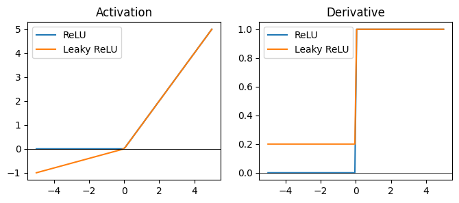
In an effort to combat the vanishing gradient problem, the next class of activations instead model a piecewise nonlinearity. The simplest of these is the rectified linear unit (ReLU) which simply takes the form:
The ReLU lets positive values through without change, and clips negative values to zero. While this ensures a well-behaved gradient at all points, the gradient at negative values is zero, which potentially slows down learning. The leaky ReLU uses a constant multiplier on the negative portion rather than a hard clip.
def relu(x):
    return jnp.maximum(0, x)
def leaky_relu(x):
    return jnp.maximum(0.2 * x, x)

plot_activations([relu, leaky_relu], ['ReLU', 'Leaky ReLU'])
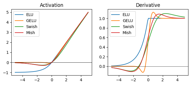
The ReLU family is highly effective, and in most models today use some variants of the ReLU activation. More modern activation functions attempt to address certain theoretical problems with the naive ReLU. Exponential linear unit (ELU) uses a saturating function that is lower bounded to (-1, inf).
Several activation functions introduce a non-monoticity property, such that the activation has a small dip near zero. This is argued to increase expressivity and gradient flow. Examples of such functions are the Gaussian error linear unit (GELU), Swish, and Mish. Swish and Mish are referred to as self-gating activation functions, as they take the form f(x) = x * gate(x), where gate(x) is a squashed function.
def elu(x):
    return jnp.where(x > 0, x, jnp.exp(x) - 1)
def gelu(x):
    return 0.5 * x * jax.lax.erfc(-x / jnp.sqrt(0.5))
def swish(x):
    return x * sigmoid(x)
def mish(x):
    return x * jnp.tanh(jnp.log(1 + jnp.exp(x)))
plot_activations([elu, gelu, swish, mish], ['ELU', 'GELU', 'Swish', 'Mish'])