Normalization Functions

Normalization functions are placed between layers to ensure that intermediate features stay within a reasonable range.

Under normal assumptions, we have no guarantees that the features at each layer are well-behaved. For numerical reasons, we often would like all our features to be normalized in some way, to maintain a mean of zero and unit variance. To achieve this property, we often insert normalization functions at key stages within the neural network.

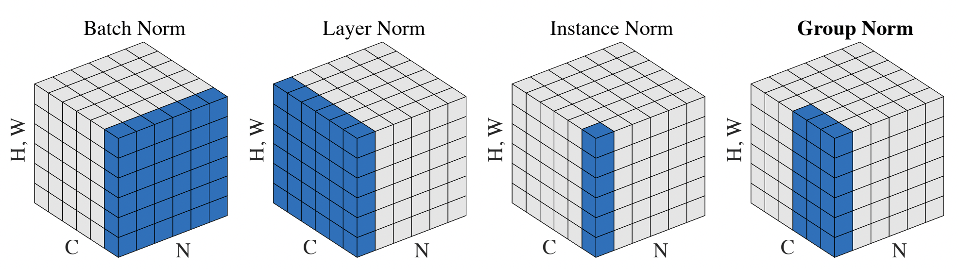
Source: Wu and He, 2018. Various normalization schemes.

Batch Norm

The first proposed technique was batch norm, which attempts to normalize the expectation of a given feature under the entire batch. To do this, we can simply calculate the mean and standard deviation of each feature elementwise, then divide the features by these statistics when passing through the batch norm layer. The downside of batch norm is the dependency on a large enough batch – at small batch sizes, the calculated mean/variances may be inaccurate. Also, we need to know what to do at inference time – typically, we would keep a running average of the mean/stddev of each feature during training, then normalize by these values during test time.

Why can’t we use the running average during training? An astute reader will ask why we can’t use our high-accuracy averages during training. The catch is we need to backprop through the normalization. Let’s assume that the gradient of a particular feature points towards increasing its value. If the normalization statistics are treated as a constant, then this gradient will be unchanged. However, if the statistics are themselves included in the gradient update, then gradient update will take the normalization into account and avoid naively increasing the feature value.

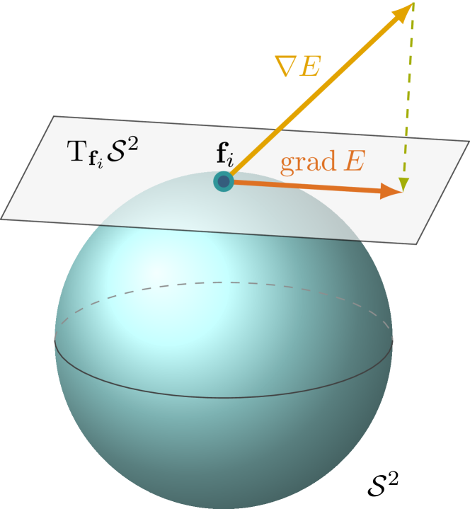
Source: Sutti and Yueh 2024. When normalization is included in gradient calculation, the gradient will be tangent on the constraint surface (sphere).

x = np.random.randn(1000, 100) * 10 # Batch of 1000, with 100 features each.
x += np.arange(100) # Add some per-feature correlations.
print('(Un-normalized) Average std per feature:', jnp.mean(jnp.std(x, axis=0)))
print('(Un-normalized) Average std of feature vector:', jnp.mean(jnp.std(x, axis=1)))

def batch_norm(x):
    mean = jnp.mean(x, axis=0)[None, :]
    var = jnp.var(x, axis=0)[None, :]
    return (x - mean) / jnp.sqrt(var + 1e-5)
y = batch_norm(x)
print('Average std per feature:', jnp.mean(jnp.std(y, axis=0)))
print('Average std of feature vector:', jnp.mean(jnp.std(y, axis=1)))

(Un-normalized) Average std per feature: 10.009361
(Un-normalized) Average std of feature vector: 30.478842
Average std per feature: 1.0
Average std of feature vector: 0.99203044

Layer Norm

Motivated by a desire to remove the batch-dependent scaling, layer norm picks a different axis of normalization. Now, instead of normalizing across the batch dimension, we instead normalize across the feature dimension. This technique means that while each individual feature may not have unit variance, the total scale/variance of a feature vector will be normalized.

x = np.random.randn(1000, 100) * 10 # Batch of 1000, with 100 features each.
x += np.arange(100) # Add some per-feature correlations.
def layer_norm(x):
    mean = jnp.mean(x, axis=1)[..., None]
    var = jnp.var(x, axis=1)[..., None]
    return (x - mean) / jnp.sqrt(var + 1e-5)
y = layer_norm(x)
print('Average std per feature:', jnp.mean(jnp.std(y, axis=0)))
print('Average std of feature vector:', jnp.mean(jnp.std(y, axis=1)))

Average std per feature: 0.32418188
Average std of feature vector: 1.0

Instance Norm

Instance norm is only relevant in convolutional networks, which have an additional (height * width) dimension in their features. Transformers today also have an additional (sequence length) dimension, so in principle one can use instance norm there. Let’s call this the parallel dimension, and consider feature tensors of the form (batch, parallel, num_features). The idea here is to normalize individual feature statistics, but within the parallel dimension rather than the batch dimension. This way we can be batch-agnostic, but still properly normalize.

x = np.random.randn(1000, 200, 100) * 10 # Batch of 1000, with 200 parallel, with 100 features each.
x += np.arange(100)[None, None, :] # Add some per-feature correlations.
x += np.arange(200)[None, :, None] # Add some per-parallel correlations.
def instance_norm(x):
    mean = jnp.mean(x, axis=1)[:, None, :]
    var = jnp.var(x, axis=1)[:, None, :]
    return (x - mean) / jnp.sqrt(var + 1e-5)
y = instance_norm(x)
print('Average std per feature:', jnp.mean(jnp.std(y, axis=(0,1,2))))
print('Average std of feature vector:', jnp.mean(jnp.std(y, axis=(0,1))))
print('Average std within parallel axis:', jnp.mean(jnp.std(y, axis=(0,2))))

Average std per feature: 0.99999976
Average std of feature vector: 1.0
Average std within parallel axis: 0.16981931

Group Norm

In between instance norm and layer norm is group norm. The idea here is to normalize all features within the parallel axis (same as instance norm), but also within an N-sized group along the feature dimension. Group norm allows for there to be additional normalization dependencies between certain feature groups.

x = np.random.randn(1000, 200, 100) * 10 # Batch of 1000, with 200 parallel, with 100 features each.
x += np.arange(100)[None, None, :] # Add some per-feature correlations.
x += np.arange(200)[None, :, None] # Add some per-parallel correlations.
def group_norm(x):
    mean = jnp.mean(x, axis=1)[:, None, :]
    var = jnp.var(x, axis=1)[:, None, :]
    x = (x - mean) / jnp.sqrt(var + 1e-5)
    num_groups = 10
    xg = x.reshape(x.shape[0], x.shape[1], num_groups, -1)
    group_means = jnp.mean(xg, axis=2, keepdims=True)
    group_vars = jnp.var(xg, axis=2, keepdims=True)
    return ((xg - group_means) / jnp.sqrt(group_vars + 1e-5)).reshape(x.shape)
y = group_norm(x)
print('Average std per feature:', jnp.mean(jnp.std(y, axis=(0,1,2))))
print('Average std of feature vector:', jnp.mean(jnp.std(y, axis=(0,1))))
print('Average std within parallel axis:', jnp.mean(jnp.std(y, axis=(0,2))))

Average std per feature: 0.999752
Average std of feature vector: 0.99975175
Average std within parallel axis: 0.9997527

Weight Norm

Another approach is to use weight norm, which does not operate on features but instead the raw parameter matrices. Here, we need to assume that the inputs to the dense layer are already normalized – we just want to make sure that they remain normalized as outputs. We can do this by normalizing the dense parameter matrix across the feature dimension. Each feature is therefore an RMSNorm-1 function of its inputs.

x = np.random.randn(1000, 100) * 10 # Batch of 1000, with 100 features each.
x += np.arange(100) # Add some per-feature correlations.
x = (x - jnp.mean(x, axis=0)) / jnp.std(x, axis=0) # Normalize.

W = np.random.randn(100, 50) / np.sqrt(100)
W += np.arange(50)[None, :] # Add some per-feature correlations.
y = x @ W
print('(Un-normalized) Average std per feature:', jnp.mean(jnp.std(y, axis=0)))
print('(Un-normalized) Average std of feature vector:', jnp.mean(jnp.std(y, axis=1)))

def weight_norm(w):
    return w / jnp.linalg.norm(w, axis=0, keepdims=True)
Wp = weight_norm(W)
yp = x @ Wp
print('Average std per feature:', jnp.mean(jnp.std(yp, axis=0)))
print('Average std of feature vector:', jnp.mean(jnp.std(yp, axis=1)))

(Un-normalized) Average std per feature: 241.60356
(Un-normalized) Average std of feature vector: 112.21661
Average std per feature: 0.9859988
Average std of feature vector: 0.16107996

Is weight norm the same as any of the previous normalization layers? No. The simple example is if an input to the dense layer has a magnitude of 1000. Activation-based norms will handle this properly, and scale down the resulting outputs. But weight norm will preserve the norm of the input vector.

Does weight norm always preserve the norm of the input vector? Again, no. Weight norm will preserve the norm of the input in expectation, assuming each coordinate of the input is independent. However, if the input vector happens to correctly align with the parameter matrix, then the norm of the output can increase. Here is an example:

def rms_norm(x, axis=-1):
    return jnp.sqrt(jnp.sum(jnp.square(x), axis=axis))

print('Independent inputs and parameters.')
x = np.random.randn(1000, 100) / np.sqrt(100)
W = np.random.randn(100, 100)
Wp = weight_norm(W)
yp = x @ Wp
print('Average RMSNorm of input vector:', jnp.mean(rms_norm(x, axis=1)))
print('Average RMSNorm of output vector:', jnp.mean(rms_norm(yp, axis=1)))

print('*Aligned* inputs and parameters.')
x = np.zeros((1000, 100))
x[:, 0] = 1 ,
W = np.zeros((100, 100))
W[0, :] = 1
Wp = weight_norm(W)
yp = x @ Wp
print('Average RMSNorm of input vector:', jnp.mean(rms_norm(x, axis=1)))
print('Average RMSNorm of output vector:', jnp.mean(rms_norm(yp, axis=1)))

Independent inputs and parameters.
Average RMSNorm of input vector: 0.9961614
Average RMSNorm of output vector: 0.9954167
*Aligned* inputs and parameters.
Average RMSNorm of input vector: 1.0
Average RMSNorm of output vector: 10.0

For independent inputs, the RMS norm is preserved via weight normalization. For aligned inputs, the RMS norm of the output increases to 10. This example shows an inherent tension in activation-unaware normalization – The product of norm-1 inputs and norm-1 weights is a norm-1 output if they are independent. In the worst case, the output can have a norm of sqrt(n).

This behavior is actually an example of why picking the correct matrix norms is important. The Frobenius norm of a matrix is equivalent to its RMS norm (if seen as a vector), and is the square root of the sum of squared singular values. When we perform weight normalization on a matrix, we set its Frobenius norm to 1. However, the spectral norm of a matrix is its maximum singular value. In the worst case, a matrix with Frobenius norm of 1 can have a spectral norm of sqrt(n), which is realized when the input vector perflect aligns with this largest singular vector.