PSGD and Relative Gradients#
This is a draft (Nov 5 2025)..
Preconditioned Stochastic Gradient Descent (PSGD) is a family of methodology for fitting preconditioners to neural networks. In contrast to closed-form methods, PSGD poses preconditioner fitting as an optimization problem, and uses iterative gradient descent to fit this “meta” objective. The most interesting aspects of PSGD, in my opinion, lies in the machinery used to optimize preconditioners over Lie groups, and via relative gradient descent.
For our purposes, we will focus on the whitening formulation of PSGD, also known as the Fisher criterion. Our goal is to learn a per-layer matirx \(P\) that minimizes the objective:
where \(g\) is a sampled gradient vector, and \(v\) is a random vector from the normal distribution.
There is an analytical solution to this cost function. Rearranging terms, we get:
which is precisely the whitening metric.
Of course, it is possible to use the analytical solution to \((gg^T)^{-0.5}\) and get an answer that way. But this involves an expensive matrix inversion, and would need to be re-computed as additional \(gg^T\) is updated. Instead, let’s look at alternatives that locate the solution in an iterative way.
First, let us acknowledge that \(P\) must be symmetric and positive semi-definite. Thus, a natural parameterization for \(P\) is:
We can now write down the gradient of \(cost(P)\) in terms of \(Q\).
A simple thing to do is to iteratively update \(Q\) with this gradient. Let’s see how this procedure performs. We will consider a distribution \(g\) sampled from a tri-diagonal covariance matrix:
rng = jax.random.PRNGKey(0)
d = 32

# Tri-diagonal covariance matrix.
Cov = jnp.eye(d)
Cov = np.zeros((d, d))
for i in range(d):
    Cov[max(i - 1, 0), i] = 0.5
    Cov[i, max(i - 1, 0)] = 0.5
    Cov[i, i] = 1
g_all = jax.random.multivariate_normal(rng, jnp.zeros(d), Cov, (100_000,))
print(Cov[:5, :5])
[[1.  0.5 0.  0.  0. ]
 [0.5 1.  0.5 0.  0. ]
 [0.  0.5 1.  0.5 0. ]
 [0.  0.  0.5 1.  0.5]
 [0.  0.  0.  0.5 1. ]]
From this distribution, we will fit \(P\) over two settings:
Where we can utilize the true distribution of \(gg^T\), i.e. we know
Covexplicitly.Where we can only utilize samples of \(g\), specifically, a batch of 256 samples per iteration. This will measure the robustness of our procedure in handling stochastic noise.
Show code cell content
def matrix_power(mat, power):
    u, s, vt = jnp.linalg.svd(mat)
    s_power = jnp.diag(s ** power)
    return u @ s_power @ vt

Cov_sqrt = matrix_power(Cov, 0.5)
def true_loss(P):
    error = P @ Cov_sqrt - jnp.eye(d)
    return jnp.sqrt(jnp.sum(jnp.square(error)))

@functools.partial(jax.jit, static_argnames=['batch_size'], static_argnums=[0])
def wrap_random_ggT(f, Q, g_all, rng, lr, batch_size=256):
    rng, key = jax.random.split(rng)
    g = jnp.take(g_all, jax.random.randint(key, (batch_size,), 0, g_all.shape[0]), axis=0)
    ggT = g.T @ g / batch_size
    return f(Q, ggT=ggT, lr=lr), rng

def run_with(step_fn, lr, T, random_ggT=False):
    rng = jax.random.PRNGKey(0)
    Q = np.eye(d)
    losses = []
    for i in range(T):
        if random_ggT:
            Q, rng = wrap_random_ggT(step_fn, Q, g_all, rng, lr)
        else:
            Q = step_fn(Q, ggT=Cov, lr=lr)
        if i % 1000 == 0:
            P = Q.T @ Q
            losses.append(true_loss(P))
    losses = [10 if x in (np.nan, np.inf) else x for x in losses]
    return losses

def plot_performance(step_fn, lrs_true, lrs_sampled, title, T=10_000):
    fig, axs = plt.subplots(1, 2, figsize=(8, 3))
    for lr in lrs_true:
        losses = run_with(step_fn, lr=lr, T=T)
        axs[0].plot(np.arange(len(losses)) * 1000, losses, label='LR={}'.format(lr))
    axs[0].legend()
    axs[0].set_yscale('log')
    axs[0].set_ylim(1e-5, 10)
    axs[0].set_title(f'{title}, true E[ggT]')

    for lr in lrs_sampled:
        losses = run_with(step_fn, lr=lr, T=T, random_ggT=True)
        axs[1].plot(np.arange(len(losses)) * 1000, losses, label='LR={}'.format(lr))
    axs[1].legend()
    axs[1].set_yscale('log')
    axs[1].set_ylim(1e-5, 10)
    axs[1].set_title(f'{title}, with sampled E[ggT]')

def compare_performances(step_fn_1, lr_true_1, lr_sampled_1, title1,
                         step_fn_2, lr_true_2, lr_sampled_2, title2, T=10_000):
    fig, axs = plt.subplots(1, 2, figsize=(8, 3))
    losses_true_1 = run_with(step_fn_1, lr=lr_true_1, T=T)
    losses_true_2 = run_with(step_fn_2, lr=lr_true_2, T=T)
    axs[0].plot(np.arange(len(losses_true_1)) * 1000, losses_true_1, label=title1)
    axs[0].plot(np.arange(len(losses_true_2)) * 1000, losses_true_2, label=title2)
    axs[0].legend()
    axs[0].set_yscale('log')
    axs[0].set_ylim(1e-5, 10)
    axs[0].set_title('True E[ggT]')

    losses_sampled_1 = run_with(step_fn_1, lr=lr_sampled_1, T=T, random_ggT=True)
    losses_sampled_2 = run_with(step_fn_2, lr=lr_sampled_2, T=T, random_ggT=True)
    axs[1].plot(np.arange(len(losses_sampled_1)) * 1000, losses_sampled_1, label=title1)
    axs[1].plot(np.arange(len(losses_sampled_2)) * 1000, losses_sampled_2, label=title2)
    axs[1].legend()
    axs[1].set_yscale('log')
    axs[1].set_ylim(1e-5, 10)
    axs[1].set_title('With sampled E[ggT]')
@jax.jit
def psgd_step_naive(Q, ggT, lr=0.001):
    Q_inv = jnp.linalg.inv(Q)
    delta = 2 * (Q @ ggT - Q_inv.T @ Q_inv @ Q_inv.T)
    Q = Q - lr * delta
    return Q

plot_performance(psgd_step_naive,
                 lrs_true=[0.3, 0.1, 0.03, 0.01],
                 lrs_sampled=[0.1, 0.03, 0.01, 0.003, 0.001],
                 title='PSGD Naive')
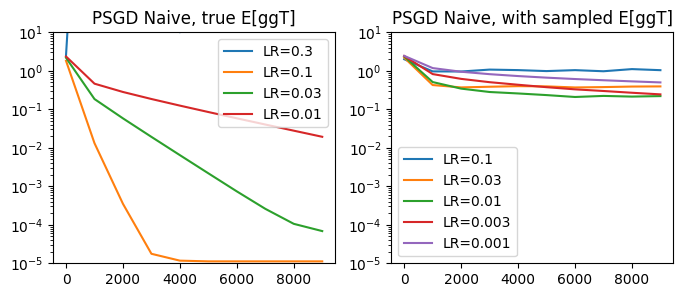
Not bad! When using the true \(ggT\) distribution, we’re able to fit to a very accurate resolution. With the sampled gradients, our solution is not as accurate, but we do see a steady gain in accuracy.
Lie Groups#
Let’s now take a step back and cover a more fundamental concept – the Lie group. While in general Lie groups are defined over abstract spaces, we will focus on Lie groups that can be embedded in real maatrices, often called matrix Lie groups. In short, a Lie group is a subset of the real invertible matrices that is closed under multiplication.
Common examples of Lie groups are set the set of diagonal matrices, the set of orthogonal matrices, or the set of matrices with determinant one. The most general matrix Lie group is the “general linear” group, which is simply the full set of invertible real matrices.
Lie group operations. Let’s start with a simple example, the group of 2x2 rotation matrices. We know that this is a subspace that is parameterized by a single parameter, \(\theta\), and in fact we know the analytic mapping:
Clearly, adding two rotation matrices does not work. However, multiplying two rotation matrices is perfectly valid, and we would end up with another rotation matrix. This shows that the 2x2 rotation matrices form a Lie group (the other requirement is that an inversion exists, which we know exists as \(R(-\theta)\), and that both of these are smooth mappings.)
The key concept is that the parameter space (\(\theta\)) is a linear basis for the multiplicative operations in group space. In our case this is understood as:
Another simple Lie group is the set of positive real numbers, which we will call \(y\). The parameter space in this case is the set of all real numbers \(x\), and the mapping between the two is the exponential function:
In fact, the concept of an exponential map is tied deeply with the idea of Lie groups. Exponential functions satisfy a key property, \(\exp(0) = 1\), which must be true for any Lie group mapping. Our matrix rotation mapping is also an exponential map, this time using the matrix exponential. Setting \(X\) as a space of 2x2 skew-symmetric matrices:
we get the relations:
Naturally, Lie groups generalize to parameter spaces that are n-dimensional. In general, a Lie group is always equipped with a Lie algebra, which is a linear basis of possible transformations. In our rotation example, the Lie algebra is the set of 2x2 skew-symmetric matrices (or equivalently, the parameter \(\theta\)). For the group of 3D rotation matrices, the Lie algebra would be the set of 3x3 skew-symmetric matrices (or equivalently, three rotation angles \(\theta_x\), \(\theta_y\), and \(\theta_z\)). The exponential map tells us how to relate a point in the Lie algrebra to a transformation in the Lie group.
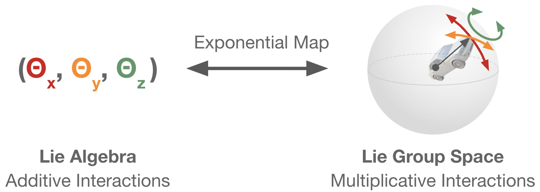
While Lie algebras are a nice way to think about the underlying behavior of Lie groups, the exponential map is often expensive to calculate and may not have a closed form. Additionally, the exponential map is at times surjective (many-to-one). So if we can, we would prefer to manipulate points on the Lie group directly. We will now examine a methodology for moving along the Lie group manifold directly via gradient descent.
Gradient Descent over Lie Groups#
Let’s now generalize the notion of gradient descent to descent within a Lie group. In classical gradient descent, we locate the steepest additive transformation, and iteratively take a step in that direction. To translate this concept to Lie groups, we will instead locate the steepest multiplicative update, or equivalently, the steepest direction on the Lie group manifold. Re-using our cost function from earlier, we will consider a matrix parameter \(Q\). Previously, we defined a small change in \(Q\) as \(dQ\), and expressed the corresponding change in the cost function in terms of \(dQ\):
Review: Additive gradient. To recover our normal additive gradient, we will explicitly go over steps that are so simple that we tend to skip over these entirely. We can first define our small delta in \(Q\) in terms of some small change \(\mathcal{E}\).
and thus the corresponding steepest descent direction in \(\mathcal{E}\) is simply:
and gradient descent is applied as:
Multiplicative (relative) gradient. Now let’s derive the update where \(Q\) is a point on the general linear Lie group (the group of all invertible matrices). The general linear Lie group is defined by all matrices \(Q\) of the form:
where \(X\) is any real matrix. The space spanned by \(X\) is often referred to as the group generator, as any group element can be produced by selecting an appropriate \(X\) and applying the exponential map. For certain Lie groups, the group generator requires a specific constraint, but for the general linear group, any real matrix \(X\) is valid. Recall that adjustments on the Lie group are defined by multiplicative interactions. We can define a small change \(\hat{dQ}\) via multiplication of \(Q\):
Here, \(\hat{\mathcal{E}}\) represents a small multiplicative change on \(Q\). \(\hat{\mathcal{E}}\) can take on any value as long as it remains in the Lie group, so we just need to make sure \(\hat{\mathcal{E}}\) is invertible. This parameterization lets us reason about small changes on the Lie group without needing to actually identify the Lie algebra vector \(dX\).
Now, we can plug our new definition of \(\hat{dQ}\) back into our original definition of \(d \; cost(Q)\), giving a new Lie group gradient:
after which the change can be applied via a gradient update as:
If we write the Lie group update in terms of the additive update, a clear relation will emerge:
The Lie group gradient update is equivalent to right-multiplying the additive update by \(Q^T Q\). As it turns out, this relation will hold regardless of the specific cost function we use. We will also refer to this update as the relative gradient descent update.
Let’s see how well this new form does.
@jax.jit
def psgd_step_relative(Q, ggT, lr=0.001):
    Q_inv = jnp.linalg.inv(Q)
    delta = 2 * (Q @ ggT @ Q.T - Q_inv.T @ Q_inv)
    Q = Q - lr * delta @ Q
    return Q

plot_performance(psgd_step_relative,
                 lrs_true=[0.2, 0.1, 0.03, 0.01],
                 lrs_sampled=[0.1, 0.03, 0.01, 0.003, 0.001],
                 title='PSGD Relative')
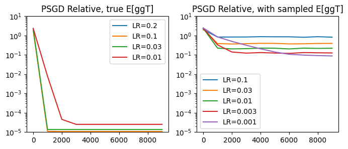
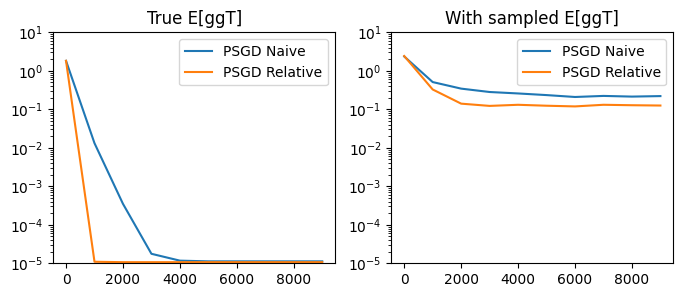
As it turns out, the relative PSGD iteration is quite powerful. Comparing the optimal learning rates between the naive and relative updates, we see that the relative update is consistently more effective:
compare_performances(
    step_fn_1=psgd_step_naive, lr_true_1=0.1, lr_sampled_1=0.01, title1='PSGD Naive',
    step_fn_2=psgd_step_relative, lr_true_2=0.1, lr_sampled_2=0.003, title2='PSGD Relative'
)
Why is the relative update more efficient?#
To understand the reason why the relative update might be desirable, it can help to look at a simpler case: the scalar square-root problem. Similar to the cost function we use to get the square-root of \(E[gg^T]\), we can define a simpler cost function that has a minimum at the elementwise square-root of any value \(a\):
To examine this problem, we’ll define \(p\) as a vector initialized with all ones, and \(a = [1/16, 1/4, 4, 16]\). Let’s consider the dynamics when we optimize this cost using additive gradient descent vs. relative gradient descent. We will plot \(p/sqrt(a)\), which has an optimum at \(1\) for all values.
a = jnp.array([1/64, 1/16, 1/4, 4, 16, 64])

@jax.jit
def true_loss_fn(p, a):
    return jnp.linalg.norm(p - jnp.sqrt(a))
@jax.jit
def grad_fn(p, a):
    return 1 - a / (p * p)
@jax.jit
def grad_fn_rel(p, a):
    return grad_fn(p, a) * p**2
Show code cell content
def plot_scalar_comparison():
    x = jnp.ones_like(a).astype(jnp.float32)
    x_vals = []
    loss_vals = []
    for _ in range(100):
        x_vals.append(x / jnp.sqrt(a))
        loss_vals.append(true_loss_fn(x, a))
        g = grad_fn(x, a)
        x = x - 0.01 * g

    x = jnp.ones_like(a).astype(jnp.float32)
    x_vals_rel = []
    loss_vals_rel = []
    for _ in range(100):
        x_vals_rel.append(x / jnp.sqrt(a))
        loss_vals_rel.append(true_loss_fn(x, a))
        g = grad_fn_rel(x, a)
        x = x - 0.01 * g

    fig, axs = plt.subplots(1, 3, figsize=(10, 3))
    for i in range(len(a)):
        axs[0].plot([xv[i] for xv in x_vals], label=f'a={a[i]}')
        axs[1].plot([xv[i] for xv in x_vals_rel], label=f'a={a[i]}')
    axs[2].plot(loss_vals, label=f'Naive GD')
    axs[2].plot(loss_vals_rel, label=f'Relative GD')

    axs[0].legend()
    axs[0].set_title('P/sqrt(A), Naive GD')
    axs[0].set_ylim(0, 4)
    axs[1].legend()
    axs[1].set_title('P/sqrt(A), Relative GD')
    axs[1].set_ylim(0, 4)

    axs[2].legend()
    axs[2].set_title('Loss')
plot_scalar_comparison()
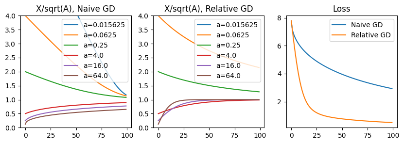
As seen above, relative gradient descent results in a descent direction that prioritizes the larger value of \(a\). This is especially important for the \(a=64\) case, which converges slowly when using naive gradient, but displays rapid convergence in the relative case. The downside of relative gradient descent appears to be slow convergence in the opposite scenario, when \(a\) is small. However, in terms of absolute contribution to the true loss on \(x\), larger terms contribute more, so this may be a bias we desire. Relative gradient desent tends to be powerful when the optimal parameters have large deviations in order-of-magnitude.
Relation to Natural Gradient Descent#
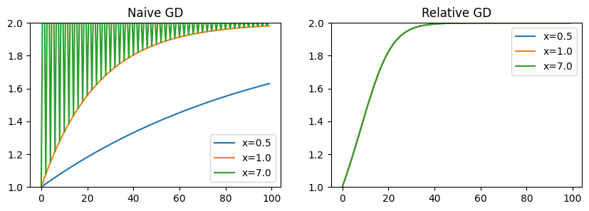
Another way to understand the relative gradient is that it represents a natural gradient descent direction for linear layers. In this case, we use “natural” not in the context of descent under the Fisher information matrix, but rather to descibe a descent direction that is invariant to parameterization. Specifically, the relative descent update will result in the same change in behavior for any \(y = Wx\), regardless of the specific structure of \(W\) or \(x\). We can show this clearly with a simple scalar example. Our loss is a simple squared loss \(L(w) = (2 - wx)^2\). If we change the input \(x\), but adjust \(w\) such that \(w/x = 1\) (i.e. \(y\) is always the same), naive gradient descent results in a varied update, while the relative update remains invariant. This means for problems where \(x\) may have a high dynamic range, the relative descent direction may result in a better-conditioned problem.
def loss_fn(w, x):
    return (2 - w*x)**2
def grad_fn(w, x):
    return 2 * jax.grad(loss_fn)(w, x)
def grad_fn_rel(w, x):
    return grad_fn(w, x) * w * w
Show code cell content
def plot_rel_comparison():
    fig, axs = plt.subplots(1, 2, figsize=(10, 3))
    for x in [0.5, 1.0, 7.0]:
        w_init = 1 / x
        y_vals = []
        for _ in range(100):
            y_vals.append(w_init * x)
            g = grad_fn(w_init, x)
            w_init = w_init - 0.01 * g
        axs[0].plot(y_vals, label=f'x={x}')

    for x in [0.5, 1.0, 7.0]:
        w_init = 1 / x
        y_vals = []
        for _ in range(100):
            y_vals.append(w_init * x)
            g = grad_fn_rel(w_init, x)
            w_init = w_init - 0.01 * g
        axs[1].plot(y_vals, label=f'x={x}')

    axs[0].legend()
    axs[0].set_title('Naive GD')
    axs[0].set_ylim(1, 2)
    axs[1].legend()
    axs[1].set_title('Relative GD')
    axs[1].set_ylim(1, 2)
plot_rel_comparison()
Inverse-Free Methods#
Let’s go back to our original loss problem of fitting the preconditioner \(P = Q^T Q\). One downside of this loss function is that it involves a matrix inverse, which is a computationally expensive operation. Recall the true loss in terms of \(Q\):
We know that using the relative gradient update, we can already remove two of the \(Q^{-1}\) terms, as multiplying the additive gradient update with \(Q^T Q\) cancels them out.
We can take this logic one step further. We can multiply the additive update by one more \(Q\) term, which removes all of the \(Q^{-1}\) terms and results in an inverse-free update:
@jax.jit
def psgd_step_invfree(Q, ggT, lr=0.001):
    delta = 2 * (Q.T @ Q @ ggT @ Q.T @ Q - jnp.eye(d))
    Q = Q - lr * delta
    return Q

plot_performance(psgd_step_invfree,
                lrs_true=[0.2, 0.1, 0.03, 0.01],
                lrs_sampled=[0.1, 0.03, 0.01, 0.003, 0.001],
                title='PSGD Inverse-Free', T=10_000)
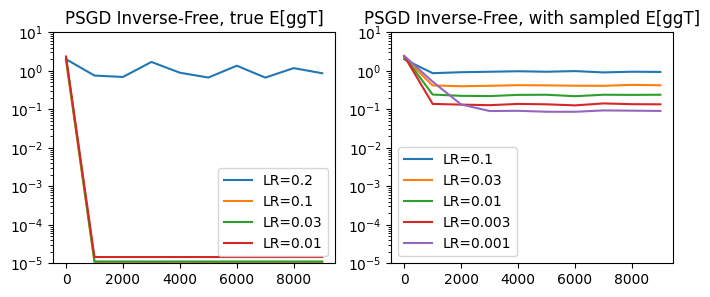
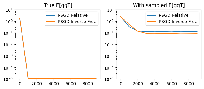
Notably, the inverse-free method tends to match the performance of the original relative update, while being much more efficient in terms of wall-clock time.
compare_performances(
    step_fn_1=psgd_step_relative, lr_true_1=0.1, lr_sampled_1=0.003, title1='PSGD Relative',
    step_fn_2=psgd_step_invfree, lr_true_2=0.1, lr_sampled_2=0.001, title2='PSGD Inverse-Free'
)

print("Timing with relative update:")
%timeit run_with(psgd_step_relative, lr=0.01, T=10_000)
print("Timing with relative inverse-free update:")
%timeit run_with(psgd_step_invfree, lr=0.01, T=10_000)
Timing with relative update:
437 ms ± 61.4 ms per loop (mean ± std. dev. of 7 runs, 1 loop each)
Timing with relative inverse-free update:
112 ms ± 1.28 ms per loop (mean ± std. dev. of 7 runs, 10 loops each)
Note: In the referenced PSGD paper, the update proposed is slightly different: they multiply by Q one more time to get:
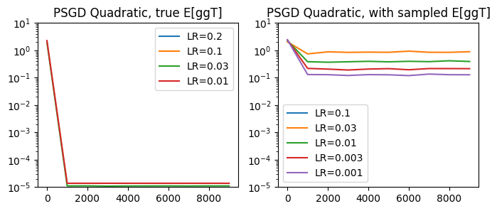
Additionally, it is stated that for the above update to be valid, \(Q\) must remain positive semi-definite. One way to ensure this is to update \(Q\) in a quadratic manner, e.g:
@jax.jit
def psgd_step_quadratic(Q, ggT, lr=0.001):
    delta = 2 * (Q.T @ Q @ ggT @ Q.T @ Q - jnp.eye(d))
    Q = (jnp.eye(d) - lr * delta) @ Q @ (jnp.eye(d) - lr * delta)
    return Q

plot_performance(psgd_step_quadratic,
                lrs_true=[0.2, 0.1, 0.03, 0.01],
                lrs_sampled=[0.1, 0.03, 0.01, 0.003, 0.001],
                title='PSGD Quadratic', T=10_000)
Connection to Newton Iteration#
We can use our machinery of relative gradients to arrive at a derivation of the well-known Newton method (sometimes called Newton-Schulz) of locating matrix inverse roots. We will repeat the above steps, this time considering \(P\) directly rather than \(Q\). Remember that \(P\) is symmetric.
and setting the update rule with a learning rate of \(1/2\):
which matches the Newton iteration for locating the inverse square-root \(A^{-0.5}\) when \(A = \mathbb{E}[gg^T]\):
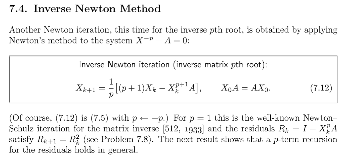
This reduces to the above equation when \(p=2\). From “Functions of Matrices”, Higham.
PSGD as an optimizer#
In this post, we specifically focused on the mechanisms of PSGD, and less on its performance as a neural network optimizer. The usage of PSGD as a competitive matrix-whitening optimizer is an open question. Computationally, PSGD has the potential to result in a much more efficient update than Shampoo/Muon as it avoids explicit matrix inversions or repeated Newton-Schulz iterations at each update.
Further Reading#
PSGD (Xi-Lin Li, there are a number of sequential papers on this):
Lie Groups:
Newton Iterations, Newton-Schulz:
Functions of Matrices, Higham: See chapters on Matrix Sign and Matrix Inverse p-th root
Relative/Natural Gradients:
Relative Gradient in Equivariant Source Separation, Cardoso and Laheld: This derives the relative gradient update.
Natural Gradient works efficiently in learning, Amari: This re-derives the \(W^T W\) update.
Adaptive Online Learning for Blind Separation, Amari: More detailed derivation of \(W^T W\).