The Transformer

The Transformer is the main architecture of choice today, combining residual connections and attention. We will implement it in 20 lines of code. Transformers are domain-agnostic and can be applied to text, images, video, etc.

History

The Transformer architecture is closely intertwined with the attention operator. Researchers working on natural language translation found that augmenting a traditional recurrent network with attention layers could increase accuracy. Later, it was found that attention was so effective, the recurrent connections could be dropped entirely – hence the title “Attention is all you need” in the original Transformer paper. Today, transformers are used not only in langauge, but across the board in image, video, robotics, and so on.

Transformer Architectural Diagram

The core of a transformer is a residual network, where each intermediate activation is a set of feature tokens. The residual blocks comprise of a self-attention layer, in which information can be shared within the set of tokens, as well as dense layers that operate independently on each token in the set.

The specific details of residual blocks vary between kinds of transformer models. We will describe the GPT-2 architecture here. In GPT-2, each residual block consists of:

• Layer norm on the residual stream vectors.

• Multi-headed self-attention.

• A residual connection, plus a second layer norm.

• Two dense layers, with a GeLU activation between.

Each attention/dense layer is applied in parallel among the entire set of feature tokens. This is why transformers can make very efficient use of GPU time – even if the global batch size is small, the effective batch size of each dense layer is batch_size * num_tokens.

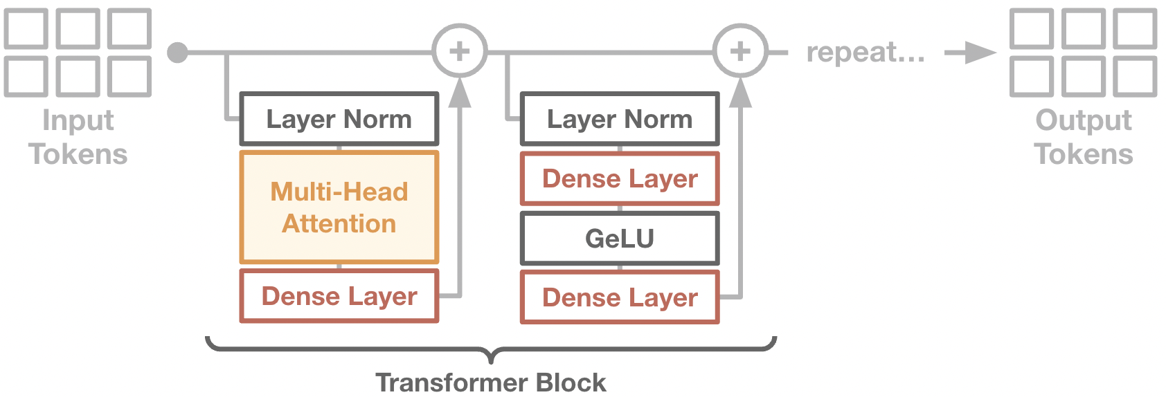
Diagram of a transformer block. Note that every operator except attention (colored background) is computed independently for each token. The attention operator is the only time in which tokens can communicate information to one another.

Many transformer implementations online come with bloated features, settings, etc. I want to stress that the core of a Transformer is incredibly simple. We can implement in only a twenty lines of code, and we will do it as follows:

class TransformerBackbone(nn.Module):
    num_features: int = 128
    num_blocks: int = 8
    num_heads: int = 4

    @nn.compact
    def __call__(self, x): # x: [batch, tokens, features]
        channels_per_head = self.num_features // self.num_heads
        for _ in range(self.num_blocks):
            # Attention block.
            y = nn.LayerNorm()(x)
            k, q, v = [nn.Dense(self.num_features)(y) for _ in range(3)]
            k, q, v = [jnp.reshape(p, (x.shape[0], x.shape[1], 
                        self.num_heads, channels_per_head)) for p in [k, q, v]]
            q = q / jnp.sqrt(q.shape[3])
            w = jnp.einsum('bqhc,bkhc->bhqk', q, k).astype(jnp.float32)
            w = nn.softmax(w, axis=-1)
            y = jnp.einsum('bhqk,bkhc->bqhc', w, q)
            y = jnp.reshape(y, x.shape)
            y = nn.Dense(self.num_features)(y)
            x = x + y
            # MLP block.
            y = nn.LayerNorm()(x)
            y = nn.Dense(self.num_features * 4)(y)
            y = nn.gelu(y)
            y = nn.Dense(self.num_features)(y)
            x = x + y
        return x
    
net = TransformerBackbone()
input = jnp.zeros((1, 10, 128))
params = net.init(jax.random.PRNGKey(0), input)['params']
output = net.apply({'params': params}, input)
print("Input shape:", input.shape)
print("Output shape:", output.shape)

Input shape: (1, 10, 128)
Output shape: (1, 10, 128)

When you look inside popular transformer implementations, at some point you will find a module that looks like the one we just defined. This transformer trunk is where the bulk of the processing and computation takes places. It is a blessing that regardless of the data type, we can use a transformer – know the transformer well, and you will be prepared for most settings.

The remaining layers of a transformer are the small input heads and output heads that surround the trunk. These heads will change based on the data format, and we will describe two common ones below.

Input Heads

Today, many have adopted the transformer as a default network architecture, regardless of domain. What remains domain-specific are the specific input and output heads required to transform the raw data into a token representation. Remember that in a transformer, the input to the network is a set of tokens – each which is a real-valued vector.

In language, the raw data is a set of words, represented as discrete integers. To turn these integers into tokens, we use an embedding layer, which is just a lookup table. Under the hood, the embedding layer is a [vocab_size, num_features] matrix. To encode a given word, we simply take the corresponding feature vector in the embedding layer matrix.

class EmbeddingInput(nn.Module):
    vocab_size: int = 256
    num_features: int = 128

    @nn.compact
    def __call__(self, x): # x is [batch, tokens (int)]
        embedding_matrix = self.param('embedding', nn.initializers.xavier_uniform(), (self.vocab_size, self.num_features))
        return jnp.take(embedding_matrix, x, axis=0)
    
net = EmbeddingInput()
input = jnp.ones((1, 10), dtype=jnp.int32)
params = net.init(jax.random.PRNGKey(0), input)['params']
output = net.apply({'params': params}, input)
print("Input shape:", input.shape)
print("Output shape:", output.shape)

Input shape: (1, 10)
Output shape: (1, 10, 128)

For images, the raw data is a 2D matrix. To transform the image into a set of tokens, we use a patch layer, which breaks up the image into non-overlapping patches, using each patch as the initialization of a token. The patch layer is often implemented as a convolutional layer, followed by a reshape to turn the 2D patches into a token set.

class PatchInput(nn.Module):
    num_features: int = 128
    patch_size: int = 16

    @nn.compact
    def __call__(self, x): # x is [batch, height, width, colors]
        patch_tuple = (self.patch_size, self.patch_size)
        num_patches = (x.shape[1] // self.patch_size)
        x = nn.Conv(self.num_features, patch_tuple, patch_tuple, padding="VALID")(x) # (B, P, P, hidden_size)
        x = rearrange(x, 'b h w c -> b (h w) c', h=num_patches, w=num_patches)
        return x
    
net = PatchInput()
input = jnp.zeros((1, 128, 128, 3))
params = net.init(jax.random.PRNGKey(0), input)['params']
output = net.apply({'params': params}, input)
print("Input shape:", input.shape)
print("Output shape:", output.shape) # 8*8 patches = 64 tokens

Input shape: (1, 128, 128, 3)
Output shape: (1, 64, 128)

Output Heads

Likewise, we also need to define output heads to project our final tokens back to the raw data format. For text or classification tasks, we generally use a classification head that maps each token into a logit vector. For image outputs, we use an patch output head, that linearly projects each token back into the original patch size. Nothing fancy here.

class ClassifierOutput(nn.Module):
    num_classes: int

    @nn.compact
    def __call__(self, x):
        return nn.Dense(self.num_classes, global_dtype)(x)

class PatchOutput(nn.Module):
    patch_size: int
    channels: int

    @nn.compact
    def __call__(self, x, c):
        batch_size, num_patches, _ = x.shape
        patch_side = int(num_patches ** 0.5)
        x = nn.Dense(self.patch_size * self.patch_size * self.channels, dtype=global_dtype)(x)
        x = jnp.reshape(x, (batch_size, patch_side, patch_side, self.patch_size, self.patch_size, self.channels))
        x = jnp.einsum('bhwpqc->bhpwqc', x)
        x = rearrange(x, 'B H P W Q C -> B (H P) (W Q) C', H=patch_side, W=patch_side)
        return x

A Unified Architecture

Today, most large-scale models use a transformer backbone. The transformer does not depend on domain-specific assumptions, which has allowed its widespread use. While there may be a shiny new architecture in the next years, the trend of a unifying architecture is likely to hold.

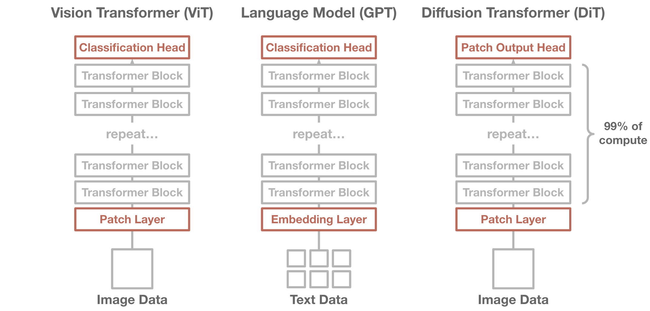
Common large-scale models today. The transformer backbone is almost identical in all settings.