Convolutional Layers

The convolutional layer is an architecture for 2D data that parallelizes computation across the 2D axes.

A typical Imagenet classification example is 224x224 pixels, with 3 color dimensions. That is a total of 150,528 input features. This size is far too much for a dense layer to be practical.

Thankfully, we can use parameter sharing to reduce parameter requirements. Parameter sharing lets us reuse parameters to process certain recurring patterns in the input. For images, we know that natural structures are largely translation-invarant – the same patterns appear at various areas of the image.

The convolution mechanism helps us formalize the notion of parameter sharing over height and width. In a convolution, we define a kernel with a size of (height, width). When applied to any (height, width) patch, the kernel outputs a linear combination of those pixels. To convolve the image with the kernel, we process the entire image by sliding the kernel (in parallel) over the entire image. A convolution shares parameters across height and width in parallel.

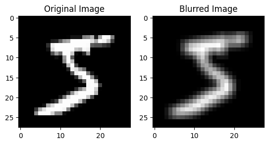
Example: Blur Convolutional Kernel

To show how convolution works, let’s define a simple blur kernel. Our kernel will be a 3x3 array of all ones. When we apply this kernel to the image, each output pixel will be a weighted average of the 3x3 input pixels around it.

kernel = jnp.ones((3, 3)) # 3x3 Blur Kernel
kernel = kernel / kernel.sum()

from keras.datasets import mnist
(train_images, train_labels), (valid_images, valid_labels) = mnist.load_data()
image = train_images[0:1].astype(np.float32)
image = jnp.expand_dims(image, axis=-1)

def apply_kernel(image, kernel):
    new_image = np.zeros_like(image)
    for x in range(1,image.shape[1]-1):
        for y in range(1,image.shape[2]-1):
            new_image[:, x, y] = np.sum(image[:, x-1:x+2, y-1:y+2] * kernel[None,:,:])
    return new_image

new_image = apply_kernel(image, kernel)
fig, axs = plt.subplots(1, 2)
axs[0].imshow(image[0], cmap='gray')
axs[0].set_title('Original Image')
axs[1].imshow(new_image[0], cmap='gray')
axs[1].set_title('Blurred Image')
plt.show()

Convolutional Layers in Neural Networks

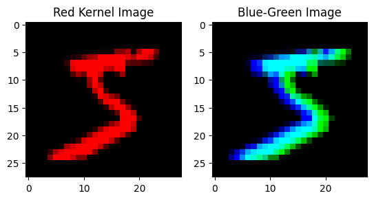
Let’s implement a simple convolutional layer in JAX. Similar to the manual example above, we’ll define a convolutional kernel, but this time over features. Our kernel will have shape (in_features, height, width, out_features), and can be thought of as a dense layer mapping from a (in_features, height, width)-size matrix input to an out_features-size vector.

Here, we’ll visualize some basic kernels by mapping from the 1-channel grayscale space to a 3-channel RGB space.

x = image / 255.0 # (1, 28, 28, 1)

def apply_kernel(x, kernel, stride=(1,1), padding='SAME'):
    x_t = jnp.transpose(x, (0, 3, 1, 2))
    kernel_t = jnp.transpose(kernel, (3, 0, 1, 2))
    y_t = jax.lax.conv(x_t, kernel_t, stride, padding)
    return jnp.transpose(y_t, (0, 2, 3, 1))

red_kernel = jnp.zeros((1, 3, 3, 3))
red_kernel = red_kernel.at[:, 1, 1, 0].set(1) # Map center to red.
x_red = apply_kernel(x, red_kernel)

bg_kernel = jnp.zeros((1, 3, 3, 3))
bg_kernel = bg_kernel.at[:, 1, 0, 1].set(1) # Map left-center to blue.
bg_kernel = bg_kernel.at[:, 1, 2, 2].set(1) # Map right-center to green.
x_blue_green = apply_kernel(x, bg_kernel)

fig, axs = plt.subplots(1, 2)
axs[0].imshow(x_red[0])
axs[0].set_title('Red Kernel Image')
axs[1].imshow(x_blue_green[0])
axs[1].set_title('Blue-Green Image')
plt.show()

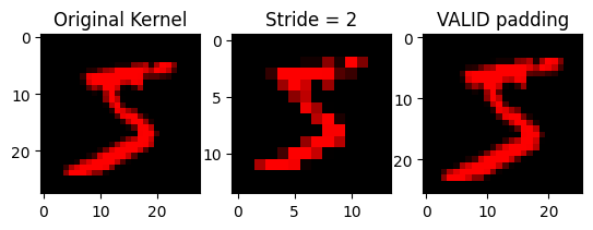
Stride and Padding

You’ll notice that our output features have the same height/width as the input features. This symmetry is not always the case, and in fact depends on two settings.

Stride is the spacing between each application of the convolution kernel. In the examples above, we used a stride of 1 to keep the height/width the same. If we use a stride of 2, the kernel will only process every other pixel, and our output will shrink by a factor of 2.

Padding is used to dictate behavior near the edges of the images. When applying a convolutional kernel to a pixel near the edge, there are no neighboring pixels past the boundary of the image. Instead, we can use the SAME strategy to pad with a copy of the center pixel, or VALID to ignore these edge cases (reducing the output size).

x_small = apply_kernel(x, red_kernel, stride=(2, 2))
x_valid = apply_kernel(x, red_kernel, padding='VALID')

fig, axs = plt.subplots(1, 3)
axs[0].imshow(x_red[0])
axs[0].set_title('Original Kernel')
axs[1].imshow(x_small[0])
axs[1].set_title('Stride = 2')
axs[2].imshow(x_valid[0])
axs[2].set_title('VALID padding')
plt.show()

Convolutional Neural Networks

A typical convolutional network will have a structure that first processes images with a series of convolutional layers, progressively decreasing the height/width dimension. This is achieved by using a stride greater than one. Eventually, these 2D feature maps are collapsed into a 1D vector for a series of dense layers.

class MyConvNet(nn.Module):

    @nn.compact
    def __call__(self, x): # Input: (B, 244, 244, 3)
        print(x.shape)
        for i in range(5):
            x = nn.Conv(features=2**(3+i), kernel_size=(3, 3), strides=(2,2))(x)
            print(x.shape)
        x = jnp.reshape(x, (x.shape[0], -1)) # (B, 15*15*128)
        print(x.shape)
        x = nn.Dense(features=10)(x)
        return x
net = MyConvNet()
params = net.init(jax.random.PRNGKey(0), jnp.zeros((1,244,244,3)))['params']
print('Parameter Kernel #4 has shape:', params['Conv_4']['kernel'].shape)

(1, 244, 244, 3)
(1, 122, 122, 8)
(1, 61, 61, 16)
(1, 31, 31, 32)
(1, 16, 16, 64)
(1, 8, 8, 128)
(1, 8192)
Parameter Kernel #4 has shape: (3, 3, 64, 128)

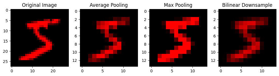
Pooling Layers

Another often-employed strategy is to pool features by hand. Instead of using convolutional kernels with a high stride, we only use stride-1 kernels. Instead, dimensionality is reduced via downsampling functions.

Given a pooling patch (usually 2x2), the simplest average pooling strategy takes the average of these features. Max pooling instead takes the maximum, which can be good for identifying high-magnitude activations. Certain architectures also use image processing techniques such as bilinear downsampling.

def average_pool(x):
    x = jnp.reshape(x, (x.shape[0], x.shape[1]//2, 2, x.shape[2]//2, 2, x.shape[3]))
    x = jnp.mean(x, axis=(2, 4))
    return x

def max_pool(x):
    x = jnp.reshape(x, (x.shape[0], x.shape[1]//2, 2, x.shape[2]//2, 2, x.shape[3]))
    x = jnp.max(x, axis=(2, 4))
    return x

def bilinear_downsample(x):
    x = jax.image.resize(x, (x.shape[0], x.shape[1]//2, x.shape[2]//2, x.shape[3]), method='bilinear')
    return x

x_average = average_pool(x_red)
x_max = max_pool(x_red)
x_bilinear = bilinear_downsample(x_red)

fig, axs = plt.subplots(1, 4, figsize=(12, 3))
axs[0].imshow(x_red[0])
axs[0].set_title('Original Image')
axs[1].imshow(x_average[0])
axs[1].set_title('Average Pooling')
axs[2].imshow(x_max[0])
axs[2].set_title('Max Pooling')
axs[3].imshow(x_bilinear[0])
axs[3].set_title('Bilinear Downsample')

Text(0.5, 1.0, 'Bilinear Downsample')

A typical convolutional network with downsampling:

class MyConvNetAvgPool(nn.Module):

    @nn.compact
    def __call__(self, x): # Input: (B, 244, 244, 3)
        print(x.shape)
        for i in range(5):
            x = nn.Conv(features=2**(3+i), kernel_size=(3, 3))(x)
            x = nn.avg_pool(x, window_shape=(2, 2), strides=(2, 2))
            print(x.shape)
        x = jnp.reshape(x, (x.shape[0], -1)) # (B, 15*15*128)
        print(x.shape)
        x = nn.Dense(features=10)(x)
        return x
net = MyConvNet()
params = net.init(jax.random.PRNGKey(0), jnp.zeros((1,244,244,3)))['params']
print('Parameter Kernel #4 has shape:', params['Conv_4']['kernel'].shape)

(1, 244, 244, 3)
(1, 122, 122, 8)
(1, 61, 61, 16)
(1, 31, 31, 32)
(1, 16, 16, 64)
(1, 8, 8, 128)
(1, 8192)
Parameter Kernel #4 has shape: (3, 3, 64, 128)

What problems are convolutional networks used in?

Typicaly problems with image inputs (although today, we can also use patch-embedding transformers). The key assumption in a convolutional layer is translation-invariance, so a convolutional network can also be used for things such as depth maps, but not for inputs that don’t have local spatial structure (like a QR code).

How are convolutional layers initialized?

The same way we would initialize a dense layer. Remember that each output feature will be a function of (height, width, input_features) inputs, so we should initialize the parameters with the square root of this total input space.